Author Archives: Peter

R – Loops

A loop is a method of repeating the same action over and over. We will separate loops into 2 types: For loops, and While loops.

For Loops are used to iterate between bounds. We declare them with an iterator variable, similar to mathematical notation (sums, products, etc.)

for(i in 1:20){print(i)} # count from 1 to 20
for(i in 20:1){print(i)} # count from 20 to 1
for(i in 10:20){print(i)} # start at 10, count to 20

In fact, we can set the bounds of the for loop to be whatever we want, going forward, backwards, or even calling variables (So long as the call returns an integer).

a = seq(1,32, by=1)     # sequence from 1 to 32
b = rep(NA, length(a))  # vector of missing values, length same as a
for(i in 1:length(a)){   # for i in 1 to 32
  b[i] = 2^(a[i])        # b[i] = 2 to the a[i]
}

On an unrelated note, b[i] is the number of unique bitstrings that can be created using i bits.

The good news is that loops are simple and easy to understand in R. the bad news, is that loops in R are slow. There are various good practices we can do to keep them running as fast as possible, but ultimately loops are really slow. In practice, in places where the slowness of loops is an issue, we have other ways of doing the same thing.

b = 2^a

This line of code will accomplish the same thing as the previous loop. Because a is a vector, each element of a will go through the mathematical function 2^a[i].

In addition, there are various methods that can be applied to complex data structures. Methods like lapply(), sapply(), mapply() allow us to do some things we would have done in a loop much faster.

While Loops, rather than using set boundaries like a for loop, use a condition to implicitly set the bounds of the loop.

x=0
while(x < 40){  # While x is less than 40
  x = x+1       # iterate x
  print(x)
}

Note that at the 40th step, the value of x was less than 40 (39). Thus, the interpreter entered the loop again, and the final outout is 40. The condition statement in the parenthesis is a boolean statement. It has only two possible values, TRUE or FALSE. You can also nest boolean statements to allow for more complicated conditions.

Because loops are relatively slow, we try to avoid them in practice. Some tasks will ultimately call for a loop, so the functionality is there.

R – Variables

R is a powerful and free statistical programming language. It runs on a wide variety of operating systems and architectures, and has a huge wealth of plugins made possible by its free nature and simple language structure. New ideas can be prototyped and pushed out very quickly, resulting in R always being on the forefront of innovation in statistics.

In order to use R, we should begin learning how to program in general. Statistical programming is about the manipulation of data (stored in variables), and the methods we use to manipulate that data. Thus, we will separate the tasks to learn into those groups.

Variables
Variables are logical names for pieces of data. Just like the use of variables in algebra, using a variable name to contain a value allows us to abstract or generalize away from the data. Variables can be given any alpha-numeric name that starts with a character, that is not already taken by methods or special names. I will separate variables into two types: simple and composite.

Simple Variables contain a single value. We can further separate these variables by the types of values they contain.

  • Boolean Variables are the simplest type of variables. They contain a single bit, and indicate a binary response. (0,1), (no,yes), (false,true) and so on. They can be declared as such:
    a = TRUE
    b = FALSE
  • Integers refer to numbers with no floating point (no decimals, no parts of numbers). Integers are used for counting, iterating. In R, it’s somewhat difficult to declare a single integer. In most cases, attempting to do so will actually declare a numeric.
  • Numerics are numbers which can potentially contain floats. They can still contain integers, though. they can be declared as such:
    a = 1
    b = 3.342
  • Characters are variables which contain non-numeric data. Most programming languages make a distinction between characters and strings, but R does not. I should specify that this non-numeric data is simply stored as non-numeric. That doesn’t mean it doesn’t contain numeric characters. They are assigned using quotation marks. R does not care if you use single or double quote marks, but in an individual assignment, you must be consistent.
    a = "a"
    b = "6"
  • Strings are variables that contain one or more characters. They are assigned identically to characters. (rather, characters in R are just strings)
    a = "abcd6"
    b = 'pretty fly for a white guy'

Composite Variables are variables that contain more than just a single data value. In R, we can create progressively more complex and layered variables ad infinitum, so it’s a bit difficult to explain complex data structures in total. I will mention a few types and show examples of how to layer them.

  • Vectors are a single-dimensional composite data structures. They will contain multiple values in order. They can contain different types of values as well. They can be used in matrix algebra, bound to matrices, or bound together to form data frames.
    a = 1:6 # creates a vector of integers.  1,2,3,4,5,6
    a = c(1:6) # creates a vector of numerics, 1,2,3,4,5,6
    a = c("a","b","6","d","feg") # creates a vector of strings
    a = c(1,2,3,"no") # creates a vector of numerics with a single string
    a = rnorm(1000,0,1) # 1000 draws from standard normal distribution
    

    We can call or manipulate explicit parts of the vector using bracket notation. Array indexing in R starts with 1 at the first character (rather than 0).

    a[2] = b

    We can also use conditional matching in the brackets. It’s important to realize that whatever is in the brackets is a vector of positions.

  • Matrices are two-dimensional composite data structures. They can be created by binding together a number of equal length vectors using the rbind() or cbind() functions, or created directly by feeding a long vector in and declaring a row or column length. In their creation we use the matrix() function. Matrices can be used in matrix algebra.
    a = matrix(c(1:20),byrow=TRUE,ncol=5)
    a = rbind(c(1:5),c(6:10),c(11:15),c(16:20))
    

    Note that elements of the matrix can be accessed with bracket notation.

    a[i,j] # Single value in i'th row, j'th column
    a[i,] # Vector of values from i'th row 
          # - Single observation about a subject
    a[,j] # Vector of values from j'th column 
          # - All observations of a given variable
    
  • Data Frames are similar to matrices in that they contain vectors of matched length. The difference is that in data frames, the columns are named and can be accessed by those names. Data frames can be assembled by putting together vectors (in this case, the default column names are the vector names), or by coercing a matrix into a data frame (in which case, the default names for the vectors are “V1”, “V2”, and so on.
    b = c(1:10) # 1 to 10
    c = c(10:1) # 10 to 1
    d = rnorm(10,0,1) # 10 draws from standard normal distribution
    a = data.frame(b,c,d) # bind vectors of equal length into data frame
    

    An advantage of data frames is that we can manipulate or insert data by calling specific names in the data frame, or using the matrix notation in brackets previously discussed. For example, if we want to add another vector to the data frame a:

    a$e = rexp(10,1) # 10 draws from exponential distribution
    a["f"] = rexp(10,1) # also 10 draws from exponential distribution
    

    We can access the column vectors of a data frame in several ways. We can call them explicitly by name using the $ notation, we can call them again explicitly by name using the bracket notation, or we can call them by position using the matrix notation. The $ notation is easiest, but the bracket notation will help you deal with poorly named variables that were previously declared.

    The default output of a read.table() function is a data frame. If we don’t get the vector names with a header, then we can specify them manually with the names() function. Alternatively, we can use the names() to read the current vector names of the data frame.

    data = read.table("https://scg.sdsu.edu/wp-content/uploads/2013/09/brain_body.txt",skip=13,header=FALSE)
    names(data) = c("Index","Brain_Weight","Body_Weight")
    

    Here data is a data frame created by the read.table() function. the names() function expects a vector of strings the same length as the number of columns. We don’t actually need the Index variable, but it is included with the table, so we need to import it before ignoring it.

  • Models are the structures generated by any of the methods we used. They too can be termed and manipulated as variables. Parts of the model can be accessed with $ notation. If you are ever confused about the structure of the object, the str() function will tell you how to access any part of the object.
    a = lm(Brain_Weight ~ Body_Weight, data = data)
    a$residuals
    str(a)
    

Coercion refers to R’s ability to coerce variables of a given type into variables of another type. For example, if you have variables of type integer, and a function expects numerics, then the integers can be easily coerced into numerics without any extra effort on the part of the programmer. Functions that expect data frames can generally be supplied with matrices (and visa-versa).

If you encounter an error in running code (and you will) where an object isn’t in the correct variable form, and isn’t being coerced properly, then you can manually coerce the object using the as.whatever() function.

a = 1:5             # a is now an integer vector
a = as.numeric(a)   # a is now a numeric vector
a = as.character(a) # a is now a character vector
a = as.matrix(a)    # a is now a character matrix 5x1
a = as.numeric(a)   # a is now a numeric matrix, 5x1
a = t(a)            # a is now a numeric matrix, 1x5
                    # t(a) takes transpose of a
a = as.vector(a)    # a is now a numeric vector
a = data.frame(a)   # a is now a single column dataframe
a = a$a             # a is back to the numeric vector
a = as.integer(a)   # a is back to the integer vector

When coercing into matrices and dataframes, R will assume that vectors are single column matrices. When there is any doubt as to your intent, R will attempt to do what makes sense. This isn’t always what you had in mind, so be cautious.

Neural Networks (R)

In this R tutorial, we are going to be training a decision tree on the “adult” dataset hosted on UCI’s machine learning repository. In this dataset, there are 15 variables, and 32561 observations. I have prepared a tutorial on how I cleaned and blocked the data to prepare it for model building. I will start this tutorial where I left off on that one. Running the script file I prepared will download the data, strip the observations with missing values, and block the data logically. It then separates the data into a training set and validation set, so that if we are so interested, later we can compare models.

source("https://scg.sdsu.edu/wp-content/uploads/2013/09/dataprep.r")

The cleaned dataset is now contained in the list variable, data. The training set is contained under data$train, and the validation set is contained under data$val. We should load the libraries for the methods we will be using. Because this will be a tutorial about neural networks, I am going to use the library nnet.

library(nnet)

nnet is the easiest to use neural network library I have found in R. It is somewhat limited in that we are limited to a single hidden layer of nodes, but there isevidence that more layers are unnecessary. While they significantly increase complexity and calculation time, they may not provide a better model.

a = nnet(income~., data=data$train,size=20,maxit=10000,decay=.001)

In this call, I am creating an nnet object, and giving it a name a. The output variable is income, and the input variables are everything that was in the data$train data frame except for income. In the formula, that’s what the ~. stands for. The data set I am using is data$train. The maximum number of iterations I will let the net train for is 10,000. We hope that it will converge reliably before reaching this.

There is no real set method of determining the number of nodes in the hidden layer. A good rule of thumb is to set it between the number of input nodes and number of output nodes. I am using 20 here, because though we have only 14 input variables, most of those input variables spawn a number of dummy variables. I increase the number of internal nodes here as an experiment to see if it will yield a better result. I encourage you to do similar testing in any modelling you do.

The decay parameter is there to ensure that the model does not overtrain.

One way we can check the output of the classifier is the confusion matrix. This is the matrix of predicted class versus the actual class. Here we check the confusion matrix on the validation set (the set we didn’t use to train the model).

> table(data$val$income,predict(a,newdata=data$val,type="class"))
   
       0    1
  0 6146  624
  1  921 1386

Another way to check the output of the classifer is with a ROC (Reciever Operating Characteristics) Curve. This plots the true positive rate against the false positive rate, and gives us a visual feedback as to how well our model is performing. The package we will use for this is ROCR.

library(ROCR)
pred = prediction(predict(a,newdata=data$val,type="raw"),data$val$income)
perf = performance(pred,"tpr","fpr")
plot(perf,lwd=2,col="blue",main="ROC - Neural Network on Adult")
abline(a=0,b=1)

Neural Network ROC (R)We should take note here that the prediction function doesn’t care where the threshold values come from. We pass the prediction function two vectors. The first vector is the vector of class probabilities, which we call threshold values. In plotting the curve, anything above the threshold is predicted as a 1, anything below is predicted as a 0. The second vector is the vector of classes. Because we are doing binary classification, the second vector must be composed of 0’s or 1’s, and the first vector must be composed of values between 0 and 1. The prediction function outputs a prediction object, which we then pass into the performance function. We specify the performance criteria we’re looking for (the ROC curve demands true positive rate “tpr”, and false positive rate “fpr”). There is then a plot command for performance objects that will automatically plot the ROC curve we’re looking for. I add in some graphical parameters (color, line width, and a title) to get the output plot.

On the ROC curve, perfect classification occurs at the upper left corner, where we have 100% true positive rate, and a 0% false positive rate. So the best classifier is the one that comes closest to here.

Typically speaking, we would choose the threshold to be the value for which we have the greatest lift over the diagonal line. That value of lift can be considered how much better we do than random guess. However, for some applications, we declare a specific level of false positives as being acceptable, and no more. So we will only consider threshold values that keep the false positive rate in the realm of acceptibility.

Additional Resources:
Wiki: Neural Networks
University of Stirling, Professor Leslie Smith: Introduction to Neural Networks
Youtube Series – CIT, I.I.T. Kharagpur, Professor S. Sengupta: Neural Networks and their Applications

Dataset: Adult (R)

This tutorial will guide you through a moderately complex data cleaning process. Data mining and data analysis are art forms, and a lot of the steps I take are arbitrary, but I will lead you through my reasoning on them. Hopefully from that you will be able see the logic and apply it in your own analyses.

The dataset I will be using for this tutorial is the “Adult” dataset hosted on UCI’s Machine Learning Repository. It contains approximately 32000 observations, with 15 variables. The dependent variable that in all cases we will be trying to predict is whether or not an “individual” has an income greater than $50,000 a year.

data = read.table("http://archive.ics.uci.edu/ml/machine-learning-databases/adult/adult.data",
		sep=",",header=F,col.names=c("age", "type_employer", "fnlwgt", "education", 
                "education_num","marital", "occupation", "relationship", "race","sex",
                "capital_gain", "capital_loss", "hr_per_week","country", "income"),
		fill=FALSE,strip.white=T)

Here is the set of variables contained in the data.

  • age – The age of the individual
  • type_employer – The type of employer the individual has. Whether they are government, military, private, an d so on.
  • fnlwgt – The \# of people the census takers believe that observation represents. We will be ignoring this variable
  • education – The highest level of education achieved for that individual
  • education_num – Highest level of education in numerical form
  • marital – Marital status of the individual
  • occupation – The occupation of the individual
  • relationship – A bit more difficult to explain. Contains family relationship values like husband, father, and so on, but only contains one per observation. I’m not sure what this is supposed to represent
  • race – descriptions of the individuals race. Black, White, Eskimo, and so on
  • sex – Biological Sex
  • capital_gain – Capital gains recorded
  • capital_loss – Capital Losses recorded
  • hr_per_week – Hours worked per week
  • country – Country of origin for person
  • income – Boolean Variable. Whether or not the person makes more than \$50,000 per annum income.

The first step I will take is deleting two variables: fnlwgt, and education_num. The reason for this is they clutter the analysis. education_num is simply a copy of the data in education, and though if we were running more advanced analysis we could weight the observations by fnlwgt, we won’t be doing that right now. So we will simply delete them from the data frame. The following code is for deleting a list element (hence the double brackets), and is the most appropriate for completely excising a variable from a data frame.

data[["education_num"]]=NULL
data[["fnlwgt"]]=NULL

Now to begin the data preparation. All the variables that were stored as text, and some that were stored as integers, will have been converted to factors during the data import. Because we’re going to be modifying the text directly, we need to convert them to character strings. We do this for all the text variables we intend to work with.

data$type_employer = as.character(data$type_employer)
data$occupation = as.character(data$occupation)
data$country = as.character(data$country)
data$education = as.character(data$education)
data$race = as.character(data$race)
data$marital = as.character(data$marital)

We should look at the relative frequency of some groups within the variables to see if we should block them.

> table(data$type_employer)

               ?      Federal-gov        Local-gov     Never-worked          Private     Self-emp-inc 
            1836              960             2093                7            22696             1116 
Self-emp-not-inc        State-gov      Without-pay 
            2541             1298               14

Given “Never worked” and “Without-Pay” are both very small groups, and they are likely very similar, we can combine them to form a “Not Working” Category. In a similar vein, we can combine government employee categories, and self-employed categories. This allows us to reduce the number of categories significantly.

data$type_employer = gsub("^Federal-gov","Federal-Govt",data$type_employer)
data$type_employer = gsub("^Local-gov","Other-Govt",data$type_employer)
data$type_employer = gsub("^State-gov","Other-Govt",data$type_employer)
data$type_employer = gsub("^Private","Private",data$type_employer)
data$type_employer = gsub("^Self-emp-inc","Self-Employed",data$type_employer)
data$type_employer = gsub("^Self-emp-not-inc","Self-Employed",data$type_employer)
data$type_employer = gsub("^Without-pay","Not-Working",data$type_employer)
data$type_employer = gsub("^Never-worked","Not-Working",data$type_employer)
> table(data$occupation)

                ?      Adm-clerical      Armed-Forces      Craft-repair   Exec-managerial   Farming-fishing 
             1843              3770                 9              4099              4066               994 
Handlers-cleaners Machine-op-inspct     Other-service   Priv-house-serv    Prof-specialty   Protective-serv 
             1370              2002              3295               149              4140               649 
            Sales      Tech-support  Transport-moving 
             3650               928              1597

On occupation, a simple way to block the categories would include blue collar versus white collar. I separate out service industry, and other occupations that I didn’t see fitting well with the other groups into their own group. It’s unfortunate that Armed Forces won’t fit well with any of the other groups. In order to get it properly represented, we can try up-sampling it when we train the model.

data$occupation = gsub("^Adm-clerical","Admin",data$occupation)
data$occupation = gsub("^Armed-Forces","Military",data$occupation)
data$occupation = gsub("^Craft-repair","Blue-Collar",data$occupation)
data$occupation = gsub("^Exec-managerial","White-Collar",data$occupation)
data$occupation = gsub("^Farming-fishing","Blue-Collar",data$occupation)
data$occupation = gsub("^Handlers-cleaners","Blue-Collar",data$occupation)
data$occupation = gsub("^Machine-op-inspct","Blue-Collar",data$occupation)
data$occupation = gsub("^Other-service","Service",data$occupation)
data$occupation = gsub("^Priv-house-serv","Service",data$occupation)
data$occupation = gsub("^Prof-specialty","Professional",data$occupation)
data$occupation = gsub("^Protective-serv","Other-Occupations",data$occupation)
data$occupation = gsub("^Sales","Sales",data$occupation)
data$occupation = gsub("^Tech-support","Other-Occupations",data$occupation)
data$occupation = gsub("^Transport-moving","Blue-Collar",data$occupation)
> table(data$country)

                         ?                   Cambodia                     Canada                      China 
                       583                         19                        121                         75 
                  Columbia                       Cuba         Dominican-Republic                    Ecuador 
                        59                         95                         70                         28 
               El-Salvador                    England                     France                    Germany 
                       106                         90                         29                        137 
                    Greece                  Guatemala                      Haiti         Holand-Netherlands 
                        29                         64                         44                          1 
                  Honduras                       Hong                    Hungary                      India 
                        13                         20                         13                        100 
                      Iran                    Ireland                      Italy                    Jamaica 
                        43                         24                         73                         81 
                     Japan                       Laos                     Mexico                  Nicaragua 
                        62                         18                        643                         34 
Outlying-US(Guam-USVI-etc)                       Peru                Philippines                     Poland 
                        14                         31                        198                         60 
                  Portugal                Puerto-Rico                   Scotland                      South 
                        37                        114                         12                         80 
                    Taiwan                   Thailand            Trinadad&Tobago              United-States 
                        51                         18                         19                      29170 
                   Vietnam                 Yugoslavia 
                        67                         16 

The variable country presents a small problem. Obviously the United States represents the vast majority of observations, but some of the groups have such small numbers that their contributions might not be significant. A way around this would be to block the countries.

data$country[data$country=="Cambodia"] = "SE-Asia"
data$country[data$country=="Canada"] = "British-Commonwealth"     
data$country[data$country=="China"] = "China"        
data$country[data$country=="Columbia"] = "South-America"     
data$country[data$country=="Cuba"] = "Other"         
data$country[data$country=="Dominican-Republic"] = "Latin-America"
data$country[data$country=="Ecuador"] = "South-America"      
data$country[data$country=="El-Salvador"] = "South-America"  
data$country[data$country=="England"] = "British-Commonwealth"
data$country[data$country=="France"] = "Euro_1"
data$country[data$country=="Germany"] = "Euro_1"
data$country[data$country=="Greece"] = "Euro_2"
data$country[data$country=="Guatemala"] = "Latin-America"
data$country[data$country=="Haiti"] = "Latin-America"
data$country[data$country=="Holand-Netherlands"] = "Euro_1"
data$country[data$country=="Honduras"] = "Latin-America"
data$country[data$country=="Hong"] = "China"
data$country[data$country=="Hungary"] = "Euro_2"
data$country[data$country=="India"] = "British-Commonwealth"
data$country[data$country=="Iran"] = "Other"
data$country[data$country=="Ireland"] = "British-Commonwealth"
data$country[data$country=="Italy"] = "Euro_1"
data$country[data$country=="Jamaica"] = "Latin-America"
data$country[data$country=="Japan"] = "Other"
data$country[data$country=="Laos"] = "SE-Asia"
data$country[data$country=="Mexico"] = "Latin-America"
data$country[data$country=="Nicaragua"] = "Latin-America"
data$country[data$country=="Outlying-US(Guam-USVI-etc)"] = "Latin-America"
data$country[data$country=="Peru"] = "South-America"
data$country[data$country=="Philippines"] = "SE-Asia"
data$country[data$country=="Poland"] = "Euro_2"
data$country[data$country=="Portugal"] = "Euro_2"
data$country[data$country=="Puerto-Rico"] = "Latin-America"
data$country[data$country=="Scotland"] = "British-Commonwealth"
data$country[data$country=="South"] = "Euro_2"
data$country[data$country=="Taiwan"] = "China"
data$country[data$country=="Thailand"] = "SE-Asia"
data$country[data$country=="Trinadad&Tobago"] = "Latin-America"
data$country[data$country=="United-States"] = "United-States"
data$country[data$country=="Vietnam"] = "SE-Asia"
data$country[data$country=="Yugoslavia"] = "Euro_2"

I tried to use a combination of geographical location, political organization, and economic zones. Euro_1 is countries within the Eurozone that I considered more affluent, and therefore people from there are probably going to be more affluent. Euro_2 includes countries within the Eurozone that I considered less affluent. These included countries that are financially troubled like Spain and Portugal, but also the Slavic countries and those formerly influenced by the USSR like Poland. Formerly British holdings that are still closely economically aligned with Britain are included under the British-Commonwealth.

We should block the education variable as well. Ultimately the goal is to shave down the number of categories in the categorical variables. For some methods this vastly simplifies the calculations, as well as to make the output more readable. I choose to block all the dropouts together. I block high school graduates and those that attended some college without receiving a degree as another group. Those college graduates who receive an associates are blocked together regardless of type of associates. Those who graduated college with a Bachelors, and those who went on to graduate school without receiving a degree are blocked as another group. Most everything thereafter is separated into its own group.

data$education = gsub("^10th","Dropout",data$education)
data$education = gsub("^11th","Dropout",data$education)
data$education = gsub("^12th","Dropout",data$education)
data$education = gsub("^1st-4th","Dropout",data$education)
data$education = gsub("^5th-6th","Dropout",data$education)
data$education = gsub("^7th-8th","Dropout",data$education)
data$education = gsub("^9th","Dropout",data$education)
data$education = gsub("^Assoc-acdm","Associates",data$education)
data$education = gsub("^Assoc-voc","Associates",data$education)
data$education = gsub("^Bachelors","Bachelors",data$education)
data$education = gsub("^Doctorate","Doctorate",data$education)
data$education = gsub("^HS-Grad","HS-Graduate",data$education)
data$education = gsub("^Masters","Masters",data$education)
data$education = gsub("^Preschool","Dropout",data$education)
data$education = gsub("^Prof-school","Prof-School",data$education)
data$education = gsub("^Some-college","HS-Graduate",data$education)
data$marital[data$marital=="Never-married"] = "Never-Married"
data$marital[data$marital=="Married-AF-spouse"] = "Married"
data$marital[data$marital=="Married-civ-spouse"] = "Married"
data$marital[data$marital=="Married-spouse-absent"] = "Not-Married"
data$marital[data$marital=="Separated"] = "Not-Married"
data$marital[data$marital=="Divorced"] = "Not-Married"
data$marital[data$marital=="Widowed"] = "Widowed"

data$race[data$race=="White"] = "White"
data$race[data$race=="Black"] = "Black"
data$race[data$race=="Amer-Indian-Eskimo"] = "Amer-Indian"
data$race[data$race=="Asian-Pac-Islander"] = "Asian"
data$race[data$race=="Other"] = "Other"

Some changes I make were simply to make the variable names more readable or easier to type. I chose to block “spouse absent”, “separated”, and “divorced” as “not married” after some initial data mining suggested they were similar in respect to income.

data[["capital_gain"]] <- ordered(cut(data$capital_gain,c(-Inf, 0, 
            median(data[["capital_gain"]][data[["capital_gain"]] >0]), 
            Inf)),labels = c("None", "Low", "High"))
data[["capital_loss"]] <- ordered(cut(data$capital_loss,c(-Inf, 0, 
            median(data[["capital_loss"]][data[["capital_loss"]] >0]), 
            Inf)), labels = c("None", "Low", "High"))

Here I block capital gains and losses, rather than do a transformation. Both variables are heavily skewed to the point that I think a numerical transformation would not have been appropriate. So I choose to block them into “None”, “Low”, and “High”. For both variables, none means they don’t play the market. Low means they have some investments. High means they have significant investments. Both gains and losses are positively associated with higher income, because if you have money in the market, odds are you have money to begin with.

It is worth noting that by doing all this blocking, we are potentially losing some information that may be relevant. In some cases this was confounding information. In others, we simply don’t have enough data within a group to make a determination about that group. So we block them with similar groups. In all cases, blocking drastically simplifies the models we use. For categorical variables, on mathematically based methods, the actual calculation sees a dummy variable for each level within a categorical variable. So for example if you have 2 categorical variables, with five and three categories respectively, the calculation will see 8 variables added to the equation. For something like this dataset where the bulk of the variables are categorical, and each of them has several levels, it’s easy to see how the number of variables in the model equation will rise. Blocking reduces this problem.

is.na(data) = data=='?'
is.na(data) = data==' ?'
data = na.omit(data)

Here I’m omitting observations or which we don’t have data in some of the variables. This is a judgement call on my part, but we only lose a couple thousand observations when we have a pool of more than thirty thousand. Some of the methods I will be using can deal with missing data, but some can not. So it’s a good idea at this point to remove observations with missing data so as to not bias any comparisons we make between the methods.

data$marital = factor(data$marital)
data$education = factor(data$education)
data$country = factor(data$country)
data$type_employer = factor(data$type_employer)
data$occupation = factor(data$occupation)
data$race = factor(data$race)
data$sex = factor(data$sex)
data$relationship = factor(data$relationship)
data$income = as.factor(ifelse(data$income==data$income[1],0,1))

At this point, I’m done modifying the categorical variables, so I’m converting them back to factors. The values for income were stored as “>50k” and “<50k". I wanted to convert them to 0's and 1's, but because of the inequality sign in the value, I could not use conditional statements. I therefore checked what the value for income in the first observation was. It happened to be "<50k". So the ifelse statement makes all cells that are equal to the value in the first cell 0, and all other cells 1. Then I convert it to a factor.

data$age = scale(data$age)
data$hr_per_week = scale(data$hr_per_week)

For the two remaining variables in the dataset, I choose to scale them. This applies a normal transformation. Each value minus its mean over the sample standard deviation. Of course, each sample will have a different mean and standard deviation, so if we wanted to apply any trained model to new data, we would have to make note of what this particular sample’s mean and standard deviation are so as to apply the same transformation. It’s worth noting that neural networks require numerical input variables to be scaled.

sample = rbinom(dim(data)[1],1,.3)
trainset = data[sample==0,]
valset = data[sample==1,]

When comparing classifiers, it’s important to have a constant sample left out that the classifier is not trained on, to see how well the trained classifier will generalize to new data. Here, I am randomly sampling approximately thirty percent of the data into a validation set that I will then use to check the accuracy of my model.

Typically for a paper I will wrap all this preparatory code into a function called dataprep(). I have provided the complete function here for your use. You can invoke it with the following code.

source("https://scg.sdsu.edu/wp-content/uploads/2013/09/dataprep.r")

The training dataset will be contained in data$train, the validation dataset will be in data$val.

Again, some of the steps I take here are completely arbitrary. I believe there’s sufficient justification for the steps I take in blocking categories here, but I must caution you that overblocking can compromise the data as you may end up removing actual signal, or valid information, within the data.

Performance of Classifiers on Dataset

I have prepared some code to demonstrate the relative performance of the classifiers named on this particular dataset, with these particular cleaning steps used. All classifiers used the same data source, the same cleaning steps. For logistic regression, we omitted the “relationship” variable during the diagnostics and model validation phase. Otherwise, the conditions were made as similar as possible.ROC_adult 
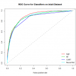
As we can see, on this dataset Random Forest has a slight early advantage, though probably not significant. Once the false positive rate gets above around .2, Logistic Regression takes over as the dominant model.

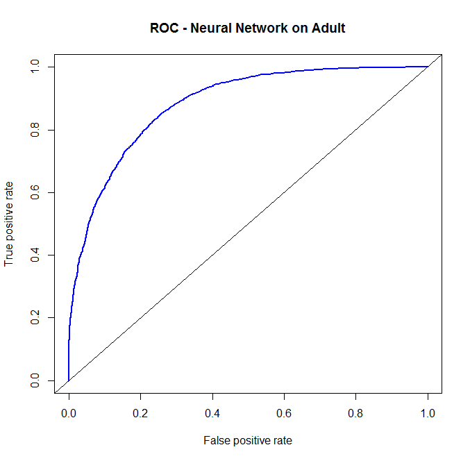
There are of course more things we can do. In much the same way bagging (by way of Random Forest) helped the CART tree, we can do the same with any other classifier. I was intentionally vague with describing the underlying classifier used in bagging, because in truth we can use any classifier with it. For instance, we can significantly improve the results of the Neural Network by bagging.

Decision Trees

Introduction to Tree Methods
Tree methods are a supervised learning method. This means that there is a pre-determined output variable (classification or regression) that we will attempt to predict.

The tree attempts to recursively partition the predictor space to model the relationship between the predictors and the response variable y. There are several advantages to trees over some other methods.

  • Trees are non-parametric, requiring few statistical assumptions
  • Trees can be applied to various data types including ordered, categorical, and continuous variables (or any combination thereof)
  • Trees perform stepwise variable selection, complexity reduction, and interaction handling in an automatic manner
  • Trees are invariant under all monotone transformations of the individual ordered predictors
  • Trees are efficient in handling missing values, and there are methods we can use to determine variable importance for the output
  • THe output is easily understood and interpreted. An individual observation follows a path through the tree that we can interpret well. This is preferable compared to “black box” methods such as Neural Networks or Support Vector Machines
  • There is a tradeoff. Trees are robust, but they are also unstable and depend heavily on the data supplied

This tutorial will cover trees as covered by “CART”, by Breiman, Friedman, Olshen and Stone (1984). This methodology addressed some of the problems of prior tree methods, and will form the foundation of some of the ensemble methods we will explore later.

Terminology

  • Trees are built from root nodes (top) to leaf or terminal nodes (bottom)
  • A record (observation) first enters the root node. A split (test) is applied to determine which child node it should go to next. This process is repeated until the record arrives at a terminal node
  • The path from the root to the leaf node provides an expression of a rule

CART Methodology
CART, standing for Classification And Regression Trees, prescribes a methdology to build and select a specific tree.

  1. Grow a large initial tree, T_0
  2. Iteratively truncat branches of T_0 to obtain a sequence of optimally pruned (nested) subtrees
  3. Select the best tree size based on validation provided by either a separate test sample (not used to build the tree), or by cross-validation (CV. Will go over later)

Grow a Large Initial Tree
To grow the initial tree, you need 4 elements.

  • A set of binary questions to induce a split
  • AA goodness of split criterion to evaluate a split
  • A stop-splitting rule
  • A rule for assigning every terminal node to a class (0 or 1)

Binary Questions
Binary questions are questions whose answers can be represented as a 0 or 1.

  • For Continuous Variables
    x>5? If yes, output 1, if no, output 0
  • For ordinal variables, we can generally regard them as continuous and treat them in the same way
  • For categorical variables, the binary question can be whether the observation belongs to a specific subset of possible values. If the possible values for x are \{a,b,c,d,e\},
    x \in a,b,d? If yes, output 1, of no, output 0

Goodness of Split Criterion
We will use a node impurity based splitting criterion to evaluate the splits. In general, the impurity i(t) can be defined as a nonnegative function of p(0|t) and p(1|t). These denote the proportions of node t beloing to classes 0,1 respectively.

    \begin{equation*} i(t) = \phi(p(y=1|t)) \end{equation*}

The impurity function is maximized when both classes are equally mixed, and is the smallest when the node contains only one class. Thus it has the following properties.

  1. \phi(p)\geq 0
  2. \phi(p) Attains minimum 0 when p=0 or p=1
  3. \phi(p) Attains its maximum when p=1-p=\frac{1}{2}
  4. \phi(p) = \phi(1-p). IE, \phi(p) is symmetric about p=\frac{1}{2}.
  5. Common choices for \phi include the Minimum Error, the Entropy function, and the Gini Index.
    Minimum or Baye’s Error

        \begin{equation*} \phi(p) = \text{min}(p,1-p) \end{equation*}

    This measure corresponds to misclassification rate when majority vote is used. This error is rarely used in practice due to its inability to sufficiently reward purer nodes.

    Entropy Function

        \begin{equation*} \phi(p) = -p\log(p) - (1-p)\log(1-p) \end{equation*}

    The entropy function is equivalent to using the likelihood ratio \chi^2 statistic for association between the branches and the target categories.

    Gini Index

        \begin{equation*} \phi(p) = p(1-p) \end{equation*}

    This is the method proposed in the original CART Method. It has been observed since that the rule has an undesireable endcut preference problem. It gives preference to the splits thatresult in two child nodes of extremely unbalanced size. To resolve this problem, a method callled the \Delta Splitting Method has been adopted in which the method will not make a cut on the last \Delta percent of the data.

    Goodness of Split Measure
    Generally speaking, the goodness of split measure is the measure of the change of node impurity. Let s e a candidate spkit and suppose s divides node t into t_L and t_R such that the proportions of cases that go into t_L and t_R are p_L and p_R repsecitvley. We can define the reduction in node impurity as

        \begin{equation*} \Delta i(s,t) = i(t)-[p_Li(t_L) + p_Ri(t_R)] \end{equation*}

    Which provides the Goodness of Split measure for s. The best split s* for node t is that which maximizes the impurity reduction.

        \begin{equation*} \Delta i(s*,t) = \max_{s\in S}i(s,t) \end{equation*}

    Then t will be split into t_L and t_R according to split s* and the search procedure will be repeated on t_L and t_R separately. A node becomes a terminal node when pre-specified terminal node conditions are satisfied.

    Tree Pruning
    Going back to the drawbacks of tree methods, trees are robust yet unstable. They heavily depend on the data that was given to them to build the tree, so they adapt to both the pattern of the data (what we want to see) and the noise of the data (what we’re trying to avoid). To obtain a tree model that can generalize well to new data, we trim back the tree iteratively to obtain a nested sequence of optimally pruned subtrees.

    Note that there exists a balance between bias and variance within tree moodels. A well fitted tree has a low bias (adapts to signal) and low variance (does not adapt to noise). For a given dataset, the more complex a tree is, the more it adapts to noise and therefore increases variance. An under-fitted tree has high bias and low variance. An overfitted tree has low bias and high variance.

    Cost Complexity Measure
    In CART, the complexity of a tree is determined by the total number of terminal nodes it has. We will again need to define some terminology:

    • Descendent and Ancestor nodes refer to the relationships between nodes. A node t is called a descendant of a higher node (ancestor node) h if there is a path leading down the tree from h to t
    • Let \tt denote the set of all terminal nodes of T, and T-\tt the set of all internal nodes of T. Furthermore, |.| denotes cardinality, IE the number of elements in the set. |\tt| represents the number of terminal nodes in tree T
    • A tree T_1 is a Subtree of T if T_1 has the same root node and T and for every node in T1, there exists the same node in T. We denote a subtree using the \succeq notation. T_1 \succeq T
    • A tree T_h is called a branch of T if T_h with root node h\in T and all descendants of h\in T are descendants of h\in T_h
    • We Prune a branch T_h off T by cutting off all descendants of the root node h in T. The pruned tree is denoted as T-T_h.
    • The Misclassification Cost of a terminal node t is given as R(t)

    WORK IN PROGRESS

    Tree Size Selection
    As the third step in the CART algorithm, we are tasked with choosing the most appropriate tree size to give the finalmodel. A natural choice is to choose the subtree that optimizes an estimate of the performance measure. However, because of the adaptive nature of trees, naively using the same data used to train the tree for testing the tree will result in an overly optimistic estimate for the performance of the model. We have a couple ways to go around this.

    Test Sample Method

    1. Split data randomly into 2 sets: L_1, the training set, and L_2, the test set
      • The ratio at which we split the data is subjective. If we have a huge amount of data, then we can afford to give a large amount (50%) to the sample set. If we have a small amount of data, we may give as little as 25% to the sample set
    2. Using the training sample L_1 only, grow a large initial tree and prune it back to obtain the nested sequence of subtrees, T_0 \succ \ldots \succ T_M
    3. Send the test sample L_2 down each subtree and compute the misclassification cost R^{ts}(T_m) based on the test sample for each subtree T_m, m=0,1,\ldots,M
      • The subtree having the smallest misclassification cost is selected the best subtree T*

            \begin{equation*} 	R^{ts}(T*) = \min_m R^{ts}(T_m) 	\end{equation*}

    4. Once the best subtree is determined, R^{ts}(T*) is used as an estimate of the misclassification cost

    There are advantages and disadvantages to the test sample method. It is very straightforward and simple. However, it does not use all the data. The sequence of subtrees, from which the best tree model is selected, is based on only part of the data.

    Cross-Validation
    Cross-validation arises to correct some of the shortcomings of the test sample method. It allows us to generate reliable out of sample error estimates without wasting data. The method explained here covers V-fold cross-validation, where we make V subsets of the data, train and calculate the out of sample error for each subset, and pick the complexity of the tree that minimizes it.

    V-fold Cross-Validation
    Whole sample L is randomly divided into V subsets. L_v, v=1,\ldots,V. The sample sizes should be approximately equal. The vth learning sample is denoted as

        \begin{equation*} L^{(v)} = L - L_v\hspace{1cm}v = 1,\ldots,V \end{equation*}

    The vth subset L_v is used as the test sample corresponding to L^{(v)}. CART suggests that we set V=10, training on 90% of the data and performing the out of sample test on 10% of the data at a time.

    1. For a fixed v, grow a large initial tree using the training set L^{(v)}. Use the pruning procedure to obtain a nested sequence of pruned subtrees, T_0^{(v)} \succ \ldots \succ T_M^{(v)}.
    2. Grow and prune a tree based on all the data to obtain the nested sequence of best-pruned subtress T_0 \succ T_1 \succ \ldots \succ T_M and the corresponding sequence of complexity parameters 0 = \alpha_0 < \ldots < \alpha_M < \alpha_M+1 = \infty
    3. Find the Complexity Parameter (CP value) associated with the minimum cross-validated misclassification cost
    4. Choose the tree associated with that CP value as the optimal tree

    In the interest of making tree models useful to new data, we may adopt a rule with regard to choosing the optimal complexity parameter. the 1-SE Rule advises us to find the complexity parameter with an associated cross-validated error less than the minimum cross-validated standard error + 1 standard deviation of that error. use of this rule is left up to the researcher. You are best off looking at a plot of tree complexity versus cross-validated error, and making your own choice.

    Additional Information
    The material contained in this section was derived from Dr. Fan’s lecture notes: ctree.pdf. These notes develop the solid mechanical underpinnings of the CART algorithm.
    See also this Youtube Presentation by mathematicalmonk.

Artificial Neural Network

Artificial Neural Networks are methods of classification and/or regression meant to emulate our belief about how a brain or nervous system functions. There exists a network of nodes, or neurons, in which various input values are calculated on. If the end value matches some condition, the neuron fires.

Network topology refers to the structure of the network. How many neurons there are, how they are arranged, and so on. The artificial neural network I will describe here is also called a Multi-Layered Perceptron. It is a layered network of perceptrons.

The Perceptron is a mathematical construct. Within the perceptron, input values are assigned weights, and then the weighted values are summed. If that sum is greater than a cutoff threshold, then the perceptron fires (Outputs a 1). Otherwise, the perceptron doesn’t fire (Outputs a 0).

    \begin{equation*} Y = \sum_{i \in 1:p}w_iX_i\hspace{1cm}\text{Output } = I(Y\geq c) = \begin{cases} 1 & Y \geq c\\ 0 & Y < c\\ \end{cases} \end{equation*}

For the first layer, the inputs to the perceptrons are the values coming from the input variables. At every layer, there is also a node with no inputs that fires an output to each of the nodes in that layer. For the second layer, and every layer thereafter, the neurons that fired will output a 1 to the next layer, while those that didn’t will output a 0.

In reality, due to the need for an activation function that is differentiable, we don’t use this identity function but rather a sigmoid function. A sigmoid function closely approximates the identity function, but is a continuous curve at all points rather than jumping at the activation threshold.

Training the ANN presents an interesting challenge. You create a cost function based on how you want the network to perform (correct classification), and the cost function increases with distance from perfect classification. In most cases, a single hidden layer will be sufficient to get the best solution for any classification problem.

Training the network means updating the various input weights to change whether the neurons fire or don’t fire. A common algorithm to do this is called the “Backpropogation” algorithm. For a given set of data, it recursively updates the weights to minimize the cost function. Each weight is an input variable to that minimization problem, so if we have a problem with 10 variables, 10 input nodes, 5 hidden nodes, and 1 output node, then we’re trying to find the global minimum of a figure in an (11 + 55 + 110) = 176 dimensional space.

The initialized weights for the untrained neural network are typically randomly drawn from a standard normal distribution. For this reason, it is important to normalize any numerical input variables so that their scale will not affect the output of the network.

Learning Rate is a value that determines how fast the neural network trains. A larger value here will cause the network to learn quickly, but it may bounce around the optimal point without reaching it.

Momentum is named so because it is similar to momentum in real life. Imagine, if you will, the current trained model is a ball, rolling down into a valley on that cost-function figure in the 176 dimensional space. Without momentum, if it reaches a local minima, it will stay there. With sufficient momentum, if it reaches a local minima, it will climb back up the hill and hopefully continue on to a global minimum. In reality, we never actually find the global minimum, we just hope the local minima we do find is comparable to it. Of course, having too much momentum will bound it out of the valley and cause us to miss the global minimum. So similar to learning rate, this is another tradeoff.

Additional Resources
Wikipedia – Artificial Neural Networks
Carlos Gershenson – Artificial Neural Networks for Beginners

Multiple Linear Regression (R)

In this tutorial, we are going to be walking through multiple linear regression, and we are going to recognize that it’s not a lot different than simple linear regression.

The model in multiple linear regression looks similar to that in simple regression. We’re adding more coefficients to modify the additional independent variables.

    \begin{equation*} Y_{i} = \beta_0 + \beta_1X_{i,1} + \beta_2X_{i,2} + \ldots + \beta_pX_{i,p} + \err_i \hspace{1cm} \err_i \sim N(0,\sigma^2) \end{equation*}

url="https://scg.sdsu.edu/wp-content/uploads/2013/09/drinking.txt"
data = read.table(url,skip=41,header=F)
names(data) = c("Index","One","pop","lb","wine","liquor","cirrhosis")

We skip the first 41 rows of the file due to it being descriptions of the data and not the data itself. Because variable names aren’t conveneniently placed on a single line, we name the columns by hand with the name() function.

We set up an ititial fit.

fit1 = lm(cirrhosis~pop+lb+wine+liquor,data=data)

To see an initial reduced model, we can use stepwise model selection to pare down the non-significant predictors. There are various criteria to determine which model we use is the “best”, but one of the more commonly used ones is Akaike’s Information Criterion, or AIC.

    \begin{equation*} \text{AIC} = 2p - 2\ln(L) \end{equation*}

Where p is the number of coefficients being calculated, and L is the maximized value of the likelihood function for the model. AIC effectively penalizes a model for using too many predictor variables, so we only include more predictor variables if they significantly increase the model’s likelihood function. That is, only if they lend sufficient additional information to the model to justify their inclusion.

library(MASS)
fit1sw = stepAIC(fit1)
summary(fit1sw)

We probably should have checked this prior to now, but it’s a good idea to check the pairwise plots of the independent versus dependent variables at some point to look for any obvious transformations we could make.

par(mfrow=c(2,2))
plot(x=data$pop,y=data$cirrhosis,xlab="population",ylab="cirrhosis")
plot(x=data$lb,y=data$cirrhosis,xlab="lower births",ylab="cirrhosis")
plot(x=data$wine,y=data$cirrhosis,xlab="wine",ylab="cirrhosis")
plot(x=data$liquor,y=data$cirrhosis,xlab="liquor",ylab="cirrhosis")

We don’t really see any obvious transformations we could make that would increase the linearity of the regressors. In like manner, there’s no obvious transformations we can make to the dependent variable to form a better regression.
As such, we have the option to stop here and take a look at the diagnostic plots of the reduced model.


Here we see the diagnostic plots of the reduced model. We don’t see any obvious pattern to the residuals, but there is some worrying deviation from the diagonal line on the QQ plot. In the Cook’s Distance plot, we’re ideally hoping that no observations have a Cooke’s Distance greater than .10. Clearly that’s not the case.

In looking at the summary of the fitted model, we can see that the final relationship given comes out to being:

    \begin{equation*} y_i = -16.0008 + 1.3656*\text{lb}_i + 1.9723*\text{wine}_i + \err_i \hspace{.5cm} \err_i \sim N(0,10.38^2) \end{equation*}

The Coefficient of Determination gives the percentage change in the dependent variable y caused by change in the independent variables lb and wine. In the summary, we see it as .8128, meaning 81% of the change in the cirrhosis variable can be “explained by” changes in the independent variables in the fit.

The F statistic is given for an overall hypothesis test,

  • H_0: \beta_i = 0 for all i. In this case, \beta_1,\beta_2 = 0, meaning that neither wine nor lb have a linear effect on cirrhosis.
  • H_1: \beta_i \neq 0 for some i. In this case, at least one of \beta_1,\beta_2 does not equal 0, meaning that there is a linear effect on cirrhosis for at least one of the predictors.

The F statistic given in the summary is 93.34, on 2 and 43 degrees of freedom. That gives a P-value very close to 0, meaning we would reject the null hypothesis. The regression is significant.

shapiro.test(fitsw$resid)

The final test for the fitted model is a test of normality of errors. The Shapiro-Wilk Normality Test will test whether the residuals of the fitted model follow a normal distribution. The hypotheses for this test are given as follows:

  • H_0: \err_i \sim N(0,\sigma^2) 
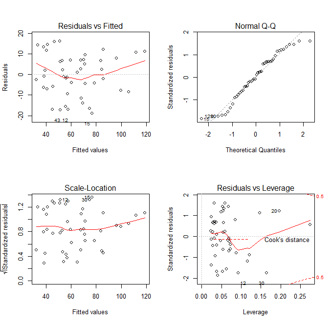
– The errors follow a normal distribution
  • H_1: \err_i \not\sim N(0,\sigma^2) – The errors do not follow a normal distribution

If we reject the null hypothesis, then we have disproved one of the base assumptions we make for linear regression. Therefore, we are hoping to not reject the null hypothesis. The output statistic from the Shapiro-Wilk test is w=.9579, with an associated p-value of .0953. Being that .0953 > .05, the \alpha level we typically use for these tests, we fail to reject the null hypothesis. We can regard the errors as normal, satisfying the assumption of the regression. We can call the fit valid.

Model Selection Schema

There are various model selection criteria in use for picking variables in linear regression. Some are applicable to other models outside of linear regression.

Akaike Information Criterion

Akaike Information Criterion, or AIC, is a measure of strength of a given model at describing the data, relative to competing models. As such, if all models fit poorly, AIC won’t give any indication of that. AIC was developed by Hirutugu Akaike, in 1974. It draws its justification from information theory.

    \begin{equation*} \text{AIC } = 2p - \ln(L) \end{equation*}

where p is the number of coefficients being calculated in the model, and L is the maximized value of the likelihood function of the model.

AIC effectively penalizes the model for having too many predictor variables. The “best fit” is the one that minimizes the AIC, because it offers the best tradeoff of maximizing the log-likelihood, and minimizing the number of predictors in the model. Additional predictors are only included if they offer enough information to justify their inclusion.

For more information, visit:

Coefficient of Determination

R^2 is the coefficient of determination. It is the percent of change in the dependent variable explained by change in the independent variables. We must first define some notation:

  • \frac{1}{n}\sum_{i=1}^n y_i = \ybar is the mean of the observed y values.
  • \yhat_i is the predicted value for the dependent variable y at the ith observation.
  • Sum of Squares – The Sums of squared values.
    • SS_{tot} = \sum_{i=1}^n(y_i - \ybar)^2 is the total deviation from mean, or total variation in the data.
    • SS_{reg} = \sum_{i=1}^n(\yhat_i - \ybar)^2 is the total variation in the regression model. This is the value we are trying to maximize, with a theoretical ceiling at SS_{tot}.
    • SS_{err} = \sum_{i=1}^n(y_i - \yhat_i)^2 is the total unexplained variation in the model. That is, the deviation from the predicted values. This is the value we are trying to minimize.

    \begin{equation*} R^2 = \frac{SS_{reg}}{SS_{tot}} =  1-\frac{SS_{err}}{SS_{tot}} \end{equation*}

R^2 is an absolute measure of “Goodness of Fit” of a model. In order to get an absolute measure of fit that penalizes high numbers of predictors, we can use the Adjusted R^2, denoted as R_{adj}^2.

    \begin{equation*} R_{adj}^2 = 1-\frac{SS_{err}/df_{err}}{SS_{tot}/df_{tot}} \end{equation*}

Where df_{err}=n-p-1, the degrees of freedom of the error term, and df_{tot}=n-1, the total degrees of freedom. (We subtract 1 degree of freedom for calculation of the mean, \ybar.)

R_{adj}^2 is a useful criterion for comparing models and determining how well a given model represents the data. It penalizes adding more predictors to the model in a similar vein to AIC, but does so in a different manner. The models selected as “best” will not necessarily be the same, and AIC is generally preferred. In some disciplines (e.g., econometrics) both of these criteria are of limited use.

For more Information, visit:

Variable Inflation Factor

The Variable Inflation Factor gives a numerical value to the severity of multicollinearity in a dataset. Multicollinearity is the degree to which some of the predictors in your dataset can be approximated as linear combinations of other predictors in your dataset. Ideally, we would have independent predictors in the dataset. Multicollinearity is the degree to which that is not the case, and VIF or Variance Inflation Factor, gives us a quantitative way of describing the Multicollinearity for a given variable.

For a given predictor variable in a predictive model, the VIF for that variable is a function of the R^2 value for a regression model predicting that variable against all other predictor variables in the predictive model. For Variable k:

    \begin{equation*} VIF_k = \frac{1}{1-R_k^2}  \end{equation*}

Where R_k^2 = R^2 of a model \hat{x}_k = \beta_0 + \beta_1x_1+\ldots+\beta_{k-1}x_{k-1}+\beta_{k+1}x_{k+1}+\ldots+\beta_px_p. The R^2 value, as the coefficient of determination, is the percent of change in the dependent variable explained by change in the predictor variables. Therefore the higher the R^2, the more the variable can be approximated by the other variables in the model. The variable inflation factor is taken as a function of this. The higher the predictive ability of the other variables on that variable, the more the variance of the coefficient of that variable is, and the more difficult the inferences made with that variable are. As a general rule, we try to omit variables with a VIF higher than 5. That may be difficult to do, so we use this as simply a guideline.

None of these regression criteria are absolute, and many times they do not agree with eachother on what the best model is. You as a statistician must use your best judgement for the model selection.

Simple Linear Regression (R)

In this tutorial we will conduct simple linear regression on a dataset on an example dataset. In the dataset there are 62 individuals, and we will be regressing brain weight over body weight. As stated before, in simple linear regression we are trying to find a linear relationship between the dependent and independent variable, that can be modeled as

    \begin{equation*} Y_i = \beta_0 + \beta_1X_i + \err_i \hspace{2cm} \err_i \sim N(0,\sigma^2) \end{equation*}

The dataset we will be using today was pulled from a set of example datasets, linked in the sample data section. I have hosted it at this website using the following URL, so you may copy and paste the code to follow along.

dataurl = "https://scg.sdsu.edu/wp-content/uploads/2013/09/brain_body.txt"
data = read.table(dataurl, skip = 12, header = TRUE)

If you visit the dataset, you will see the data does not start immediately at the first line. Because it is a text file, I have used the command read.table() to import the data. I use the skip flag to skip the first 12 rows of the file, and then set the header flag to TRUE to ensure that the variable names are taken from the first read (13th) row. So the data starts on the 14th row.

fit1 = lm(Brain_Weight ~ Body_Weight, data = data)
par(mfrow=c(1,1))
plot(x=data$Body_Weight,y=data$Brain_Weight,xlab="Body Weight",
     ylab="Brain Weight",main="Simple Linear Regression (Bad)")
abline(fit1)
par(mfrow=c(2,2))
plot(fit1)

fit1 PlotHere I create a preliminary fit, and plot the data to look at it. In fact, it was probably unnecessary to make the preliminary fit, as plotting the data we will see that it is heavily skewed and not a good candidate for regression. Observing the diagnostic plots will confirm this.
fit1 DiagnosticsIn looking at the first diagnostic plot, “Fitted vs Residuals”, we see a pattern in the residuals. This warns us of problems in the fit. In the second diagnostic plot, or “Quantile to Quantile” (QQ) plot, we see how closesly the residuals from the fit match a normal distribution. They don’t. Given that one of the assumptions of least squares linear regression is that the residuals follow a normal distribution, we can see we have a problem here.
One thing we can do to make a valid model is to attempt transformations of the variables. A reasonable choice might be a log transform of the independent variable.

fit2 = lm(Brain_Weight ~ log(Body_Weight), data = data)
par(mfrow=c(1,1))
plot(x=log(data$Body_Weight),y=data$Brain_Weight,xlab="Log(Body Weight)",
     ylab"Brain Weight",main="Simple Linear Regression (Still Bad)")
abline(fit2)
par(mfrow=c(2,2))
plot(fit2)

fit2 Plot We attempt a log transformation of the independent variable to remove some of the skew. This actually makes the fit significantly worse. Now we have a negative intercept which doesn’t make sense logically. We also see that the fitted line doesn’t follow the observations very well.

fit2 Diagnostics In looking at the diagnostic plots, we see additional problems. The QQ plot has several massive outliers, and the fitted versus residuals line has a very clear pattern. There is clearly another transformation that we haven’t done yet.

Considering that log transforming the dependent variable without transforming the independent variable would just skew the data the other way, another choice we have would be to log transform both independent and dependent variables.

fit3 = lm(log(Brain_Weight) ~ log(Body_Weight), data = data)
par(mfrow=c(1,1))
plot(log(data$Body_Weight),log(data$Brain_Weight),xlab="Log(Body Weight)",
     ylab="Log(Brain Weight)",main="Simple Linear Regression (Good)")
abline(fit3)
par(mfrow=c(2,2))
plot(fit3)

fit3 Plot
We attempt a log transform of both the independent and dependent variables. Here we can see the data nicely nested around the fitted line. This is ideally the plot we’re looking for in simple linear regression. We see a strong correllation and an interpretable relationship.

fit3 DiagnosticsObserving the diagnostic plots we see no obvious patterns in the fitted vs residual plot, and the QQ plot follows the diagonal fairly well. It diverges a bit towards the tails, so there may be a slightly better transformation we could apply, but we can regard this fit as “good enough”.

The final thing to do with this fit is test the model assumptions. We want to confirm the normality of residuals, so we’ll be applying the Shapiro-Wilk test of Normality.

In this test, our null hypothesis is that the residuals are normal, so we are hoping to NOT reject.

    \begin{align*} &H_0\text{:  The Residuals are Normally Distributed}\\ &H_1\text{:  The Residuals are not normally distributed}\\ \end{align*}

If the residuals are not normally distributed, the inferences from the regression will be meaningless. We rely on normality of errors for our inference structures (t and F tests, confidence intervals, etc.). So, applying the test to the residuals of the fit object, we get the results.

shapiro.test(fit3$residuals)

gives us the result.

> shapiro.test(fit3$residuals)

	Shapiro-Wilk normality test

data:  fit3$residuals
W = 0.9874, p-value = 0.7768

With a p-value of 0.7768 being much higher than any \alpha level we might choose to use, we will fail to reject the null hypothesis and we can regard the errors as normal. We will call this our ending model. There are various other methods we could have used to move through the models, but for simple linear regression, plotting and observing the data will give us the best idea of what is going on. We can observe the results of our regression using the summary function. From here, we can also verify that the regression is significant.

    \begin{align*} &H_0\text{:  }\beta_1 = 0\text{ - The regression is not significant}\\ &H_1\text{:  }\beta_1 \neq 0\text{ - The regression is significant}\\ \end{align*}

The test statistic for this test follows an F distribution. We will observe the results of the test from the summary output.

> summary(fit3)

Call:
lm(formula = log(Brain_Weight) ~ log(Body_Weight), data = data)

Residuals:
     Min       1Q   Median       3Q      Max 
-2.16559 -0.59763  0.09433  0.65789  2.09470 

Coefficients:
                 Estimate Std. Error t value Pr(<|t|)    
(Intercept)      -2.50907    0.18408  -13.63   < 2e-16 ***
log(Body_Weight)  1.22496    0.04638   26.41   < 2e-16 ***
---
Signif. codes:  0 ‘***’ 0.001 ‘**’ 0.01 ‘*’ 0.05 ‘.’ 0.1 ‘ ’ 1

Residual standard error: 0.8863 on 60 degrees of freedom
Multiple R-squared:  0.9208,	Adjusted R-squared:  0.9195 
F-statistic: 697.4 on 1 and 60 DF,  p-value: < 2.2e-16

R gives us an F-statistic output of 697, with an associated P-value near 0. With that we can reject the null hypothesis, and accept that there exists a linear relationship between \log(x) and \log(y). Also note that in simple linear regression with a single predictor value, the F statistic for the overall regression is the square of the t statistic for the significance of the predictor. 26.41^2 \approx 697.

Now for some math. Taking the log of both sides is in effect performing exponential regression. When we solve the revised equation for the original y, we get this.

    \begin{align*} \ln(y) &= -2.51 + 1.225\ln(x) + \err\\ e^{\ln(y)} &= e^{-2.51 + 1.225\ln(x) + \err}\\ y &= e^{-2.51}e^{\ln(x)^{1.225}}e^{\err}\\ y &= e^{-2.51 + \err}x^{1.225} \end{align*}

And this is the final relationship we arrive at with this data set.