We will apply the random forest method to the Adult dataset here.

We will begin by importing the data, doing some pre-filtering and combining into classes, and generating two subsets of the data: The training set, which we will be using to train the random Forest model, and the evaluation set, which we will use to evaluate the performance of the model.

source("https://scg.sdsu.edu/wp-content/uploads/2013/09/dataprep.r")

For more information on what this source code does to prepare the data, visit the tutorial: “Data Preparation with R (Adult Dataset)”. This allows us to move on to model specification.

Random Forests are an extension of tree methods. Where in the CART methodology, the inherent variability of the tree model, and susceptibility to data was considered a weakness of the model, in random forest that is considered a strength. In fact, we take special steps to ensure as much variability in the individual trees as possible. The belief is that by averaging across the high variance, low bias trees, we will end up with a low bias, low variance estimator. We hope that the random forest will do better than any single tree could do. We need to load up the libraries we’ll be using.

library(randomForest)
library(ROCR)

Next we’ll need to find the optimal numbers of variables to try splitting on at each node.

bestmtry <- tuneRF(data$train[-13],data$train$income, ntreeTry=100, 
     stepFactor=1.5,improve=0.01, trace=TRUE, plot=TRUE, dobest=FALSE)

For this, the syntax I’m using for the tuneRF function means I’m giving the function the first 12 columns of the training set (all values but income) as independent variables. The specification data$train[-13] means “All but the 13th column on the set data$train”. As an independent variable, I give the algorithm “data$train$income”, which is the income column on the set data$train. ntreeTry specifies the number of trees to make using this function, trying out different numbers for mtry. See the help file (help(tunerf)) for more information.

The algorithm has chosen 2 as the optimal number of mtry for each tree. Now what we have left to do is run the algorithm.

adult.rf <-randomForest(income~.,data=data$train, mtry=2, ntree=1000, 
     keep.forest=TRUE, importance=TRUE,test=data$val)

In the formula for Random Forest, we specify income versus all other variables in the set as predictors. We specify the mtry value to be 2, matching what we had found earlier with searching for the optimal value. The number of trees we use here is 1000, though computers are fast now and it’s not unreasonable to use 20,000 or more trees to build the model. We ask the algorithm to keep the forest, as well as calculate the variable importance so we can see what contributed most to estimating income classification.

Finally, we can evaluate the performance of the random forest for classification. Since we have been eschewing the confusion matrix in favor of the ROC curve, we should probably continue that. The commands to generate the ROC curve using the ROCR package are as follows:

adult.rf.pr = predict(adult.rf,type="prob",newdata=data$val)[,2]
adult.rf.pred = prediction(adult.rf.pr, data$val$income)
adult.rf.perf = performance(adult.rf.pred,"tpr","fpr")
plot(adult.rf.perf,main="ROC Curve for Random Forest",col=2,lwd=2)
abline(a=0,b=1,lwd=2,lty=2,col="gray")

To build the ROC curve using the ROCR package, first we need to generate the prediction object. As inputs to the prediction() method, we use the predicted class probabilities for the validation dataset, and the actual classes (labels). There are various things we can do with the prediction object, but the most appropriate here is to gauge the performance, using the performance() method. As inputs, we give it the performance object, and the two metrics we want to display in the ROC curve. (True positive rate, False positive rate). There are other diagnostic curves we can also generate using this method. See help(performance) for more information.

To interpret the ROC curve, let us remember that perfect classification happens at 100% True positive rate, and 0% False positive rate. With that in mind, we see that perfect classification happens at the upper left-hand corner of the graph, so the closer our graph comes to that corner, the better we are at classification. The diagonal line represents random guess, so the distance of our graph over the diagonal line represents how much better we are doing than random guess. Now we also want to evaluate what variables were most important in generating the forest.

importance(adult.rf)
varImpPlot(adult.rf)

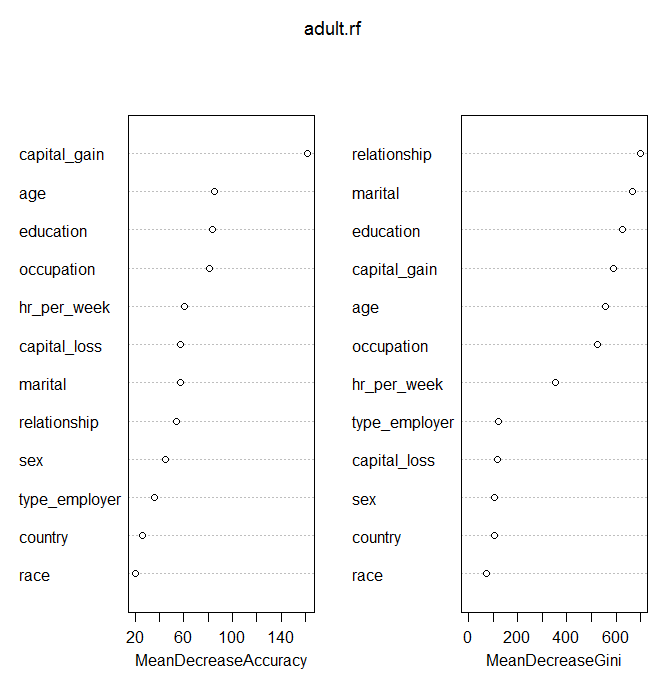The importance() function gives us a textual representation of how important the variables were in classifying income, while the varImpPlot() method gives us a graphical representation. We see from the Variable importance plot, that the most important variables included age, capital gains, education, and marital and relationship status. Variables like race and country of origin were of less importance.