Simple Linear Regression (SAS) | Statistical Consulting Group

In this tutorial we will conduct simple linear regression on a dataset on an example dataset. In the dataset there are 62 individuals, and we will be regressing brain weight over body weight. As stated before, in simple linear regression we are trying to find a linear relationship between the dependent and independent variable, that can be modeled as

$\begin{equation*} Y_i = \beta_0 + \beta_1X_i + \err_i \hspace{2cm} \err_i \sim N(0,\sigma^2) \end{equation*}$

The dataset we will be using today was pulled from a set of example datasets, linked in the sample data section. I have hosted it at this website here, so you must download the dataset to follow along. This regression will attempt to find a linear relationship between body weight, and brain weight.

FILENAME FN 'filepath\brainbody.txt';

This step isn’t really necessary, but I did want to demonstrate the ability to create filename variables to simplify subsequent proc statements.

DATA BB;              /* creating a dataset named BB         */
     INFILE FN;       /* Input File fn (declared previously) */
     INPUT INDEX BRAINWEIGHT BODYWEIGHT;/* Variables in file */
     RUN;             /* run the datastep                    */
 
DATA BB;                   /* Create a new dataset BB        */
     SET BB(DROP=INDEX);   /* Using existing set (sans index)*/
     RUN;                  /* run the datastep               */

The reason I drop the index variable is because it is unnecessary. Due to our using simple infile statements, we have to read all the data in and then drop the data we don’t need. There are more advanced input statments you could use that don’t have that limitation, but for such a small dataset this is the easiest option. Now to build a model, we use the proc reg statment.

PROC REG DATA=BB;  /*  Regression on BB Dataset             */
     MODEL BRAINWEIGHT = BODYWEIGHT; /* Brain ~ Body        */
     RUN;          /*  Run the Regression                   */

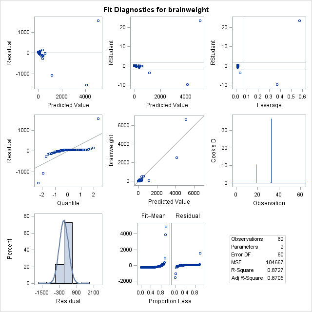By default, the proc reg statement generates quite a bit of output. The individual $t$ statistics test significance of point estimates for slope and intercept, while the $F$ statistic is the overall significance of the regression. They say that the regression is significant, so that there is a linear effect. However, none of these statistics accurately capture what is wrong with this fit. Look at the diagnostic plots, the fitted vs residual plots, and the QQ plot. They warn of something very wrong here. In the “Quantile to Quantile” (or QQ) plot, we see how closesly the residuals from the fit match a normal distribution. They don’t. Given that one of the assumptions of least squares linear regression is that the residuals follow a normal distribution, we can see we have a problem here. We can also see this by the histogram of residuals on the bottom, with a superimposed normal curve. It is clear to see that the residuals do not follow a normal distribution. To fix this, one thing we can do to make a valid model is to attempt transformations of the variables. A reasonable choice might be a log transform of the independent variable.

DATA BB;            /* Create new Dataset BB                */
     SET BB;        /* Using existing Set BB                */
     LOGBODYWEIGHT = LOG(BODYWEIGHT);
                    /* Add log transform of Bodyweight      */
     RUN;
 
PROC REG DATA=BB;   /* Run the Regression again on new BB   */
     MODEL BRAINWEIGHT = LOGBODYWEIGHT;
                    /* Brain weight Versus log(bodyweight)  */
     RUN;

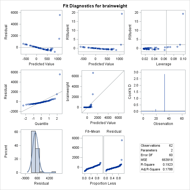We attempt a log transformation of the independent variable to remove some of the skew. In looking at the F statistic and the t-statistics for the individual $\beta$ ‘s, we can see that the regression is still significant. However, the transformation actually makes the fit significantly worse. We see a clear pattern in the residuals, and a QQ plot that appears almost flat where it should be diagonal. Considering that log transforming the dependent variable without transforming the independent variable would just skew the data the other way, another choice we have would be to log transform both independent and dependent variables.

DATA BB;             /* Create new Data-set BB              */
     SET BB;         /* Using existing set BB               */
     LOGBRAINWEIGHT = LOG(BRAINWEIGHT);
                     /* Log Transform of Brain Weight       */
     RUN;
 
PROC REG DATA=BB;   /* Create new Regression Model using BB */
     MODEL LOGBRAINWEIGHT = LOGBODYWEIGHT;
                    /* Log(Brainweight) ~ Log(BodyWeight)   */
     RUN;

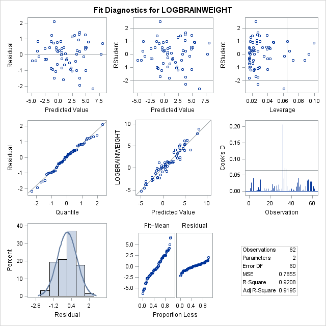We attempt a log transform of both the independent and dependent variables. Here we can see the data nicely nested around the fitted line. This is ideally the plot we’re looking for in simple linear regression. We see a strong correllation and an interpretable relationship. Observing the diagnostic plots we see no obvious patterns in the fitted vs residual plot, and the QQ plot follows the diagonal fairly well. 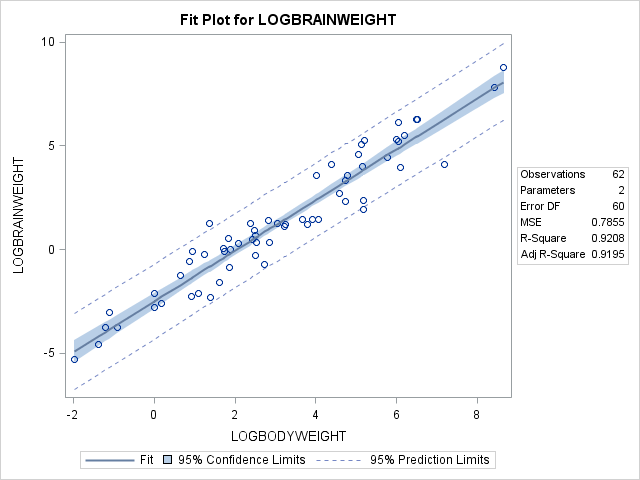It diverges a bit towards the tails, so there may be a slightly better transformation we could apply, but we can regard this fit as “good enough”.

On the fit plot, we see the 95% confidence limits, and the 95% prediction limits. This will require some explanation. Confidence Intervals refer to confidence in the parameter of the generating function. IE, we are 95% confident that the parameter that generated that data falls within that interval. They are generated as a function of the coefficient’s value and standard deviation.

Prediction limits on the other hand add in the extra variability of the error term to say that we are 95% sure that any new observation will fall within the bounds. See the theory page for the math required to generate the confidence and prediction intervals.

Now for some math. Taking the log of both sides is in effect performing exponential regression. When we solve the revised equation for the original $y$ , we get this.

$\begin{align*} \ln(y) &= -2.51 + 1.225\ln(x) + \err\\ e^{\ln(y)} &= e^{-2.51 + 1.225\ln(x) + \err}\\ y &= e^{-2.51}e^{\ln(x)^{1.225}}e^{\err}\\ y &= e^{-2.51 + \err}x^{1.225} \end{align*}$

And this is the final relationship we arrive at with this data set.

Further Reading