In this R tutorial, we are going to be training a decision tree on the “adult” dataset hosted on UCI’s machine learning repository. In this dataset, there are 15 variables, and 32561 observations. I have prepared a tutorial on how I cleaned and blocked the data to prepare it for model building. I will start this tutorial where I left off on that one. Running the script file I prepared will download the data, strip the observations with missing values, and block the data logically. It then separates the data into a training set and validation set, so that if we are so interested, later we can compare models.
source("https://scg.sdsu.edu/wp-content/uploads/2013/09/dataprep.r")
The cleaned dataset is now contained in the list variable, data. The training set is contained under data$train, and the validation set is contained under data$val. We should load the libraries for the methods we will be using. Because this will be a tutorial about neural networks, I am going to use the library nnet.
library(nnet)
nnet is the easiest to use neural network library I have found in R. It is somewhat limited in that we are limited to a single hidden layer of nodes, but there isevidence that more layers are unnecessary. While they significantly increase complexity and calculation time, they may not provide a better model.
a = nnet(income~., data=data$train,size=20,maxit=10000,decay=.001)
In this call, I am creating an nnet object, and giving it a name a. The output variable is income, and the input variables are everything that was in the data$train data frame except for income. In the formula, that’s what the ~. stands for. The data set I am using is data$train. The maximum number of iterations I will let the net train for is 10,000. We hope that it will converge reliably before reaching this.
There is no real set method of determining the number of nodes in the hidden layer. A good rule of thumb is to set it between the number of input nodes and number of output nodes. I am using 20 here, because though we have only 14 input variables, most of those input variables spawn a number of dummy variables. I increase the number of internal nodes here as an experiment to see if it will yield a better result. I encourage you to do similar testing in any modelling you do.
The decay parameter is there to ensure that the model does not overtrain.
One way we can check the output of the classifier is the confusion matrix. This is the matrix of predicted class versus the actual class. Here we check the confusion matrix on the validation set (the set we didn’t use to train the model).
> table(data$val$income,predict(a,newdata=data$val,type="class"))

       0    1
  0 6146  624
  1  921 1386
Another way to check the output of the classifer is with a ROC (Reciever Operating Characteristics) Curve. This plots the true positive rate against the false positive rate, and gives us a visual feedback as to how well our model is performing. The package we will use for this is ROCR.
library(ROCR)
pred = prediction(predict(a,newdata=data$val,type="raw"),data$val$income)
perf = performance(pred,"tpr","fpr")
plot(perf,lwd=2,col="blue",main="ROC - Neural Network on Adult")
abline(a=0,b=1)
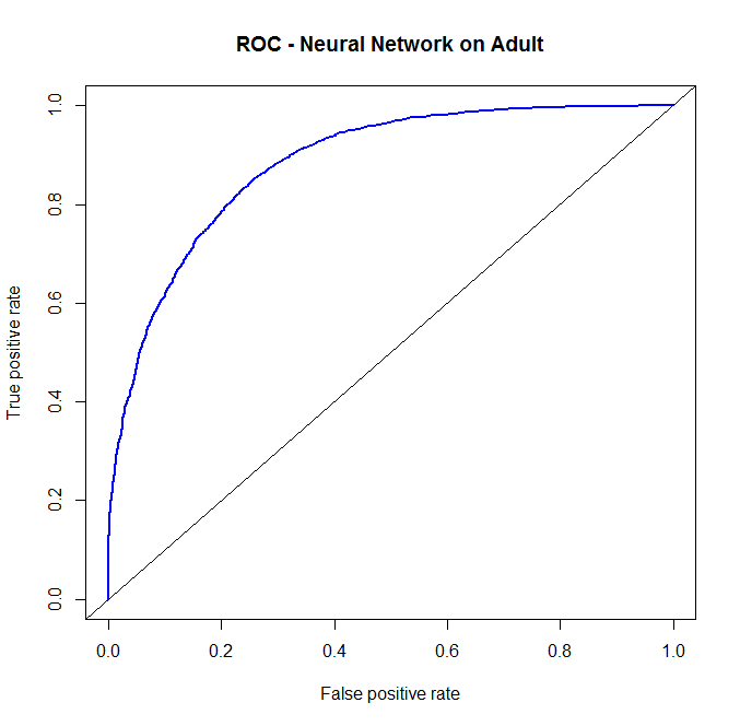 We should take note here that the prediction function doesn’t care where the threshold values come from. We pass the prediction function two vectors. The first vector is the vector of class probabilities, which we call threshold values. In plotting the curve, anything above the threshold is predicted as a 1, anything below is predicted as a 0. The second vector is the vector of classes. Because we are doing binary classification, the second vector must be composed of 0’s or 1’s, and the first vector must be composed of values between 0 and 1. The prediction function outputs a prediction object, which we then pass into the performance function. We specify the performance criteria we’re looking for (the ROC curve demands true positive rate “tpr”, and false positive rate “fpr”). There is then a plot command for performance objects that will automatically plot the ROC curve we’re looking for. I add in some graphical parameters (color, line width, and a title) to get the output plot.
On the ROC curve, perfect classification occurs at the upper left corner, where we have 100% true positive rate, and a 0% false positive rate. So the best classifier is the one that comes closest to here.
Typically speaking, we would choose the threshold to be the value for which we have the greatest lift over the diagonal line. That value of lift can be considered how much better we do than random guess. However, for some applications, we declare a specific level of false positives as being acceptable, and no more. So we will only consider threshold values that keep the false positive rate in the realm of acceptibility.
Additional Resources:
Wiki: Neural Networks
University of Stirling, Professor Leslie Smith: Introduction to Neural Networks
Youtube Series – CIT, I.I.T. Kharagpur, Professor S. Sengupta: Neural Networks and their Applications