Classification trees are non-parametric methods to recursively partition the data into more “pure” nodes, based on splitting rules. See the guide on classification trees in the theory section for more information. Here, we’ll be using the rpart package in R to accomplish the classification task on the Adult dataset. We’ll begin by loading the dataset and library we’ll be using to build the model.

source("https://scg.sdsu.edu/wp-content/uploads/2013/09/dataprep.r")
library(rpart)

The name of the library rpart stands for Recursive Partitioning. The source(“…/dataprep.r”) line runs the code located at that URL. For information in what is contained in that code, check the R tutorial on the Adult dataset. The code prepares and splits the data for further analysis.

mycontrol = rpart.control(cp = 0, xval = 10)
fittree = rpart(income~., method = "class",
     data = data$train, control = mycontrol)
fittree$cptable

If we observe the fitted tree’s CP table (Matrix of Information on optimal prunings given Complexity Parameter), we can observe the best tree. We look for the tree with the highest cross-validated error less than the minimum cross-validated error plus the standard deviation of the error at that tree. In this case, we observe the minimum cross-validated error to be 0.6214039, happening at tree 16 (with 62 splits). There we observe the standard error of that cross-validated error to be 0.01004344. We add these values together to get our maximum target error. We find the CP value for the tree with the largest cross-validated error less than 0.6314473. This occurs at tree 8, with 11 splits.

cptarg = sqrt(fittree$cptable[7,1]*fittree$cptable[8,1])
prunedtree = prune(fittree,cp=cptarg)

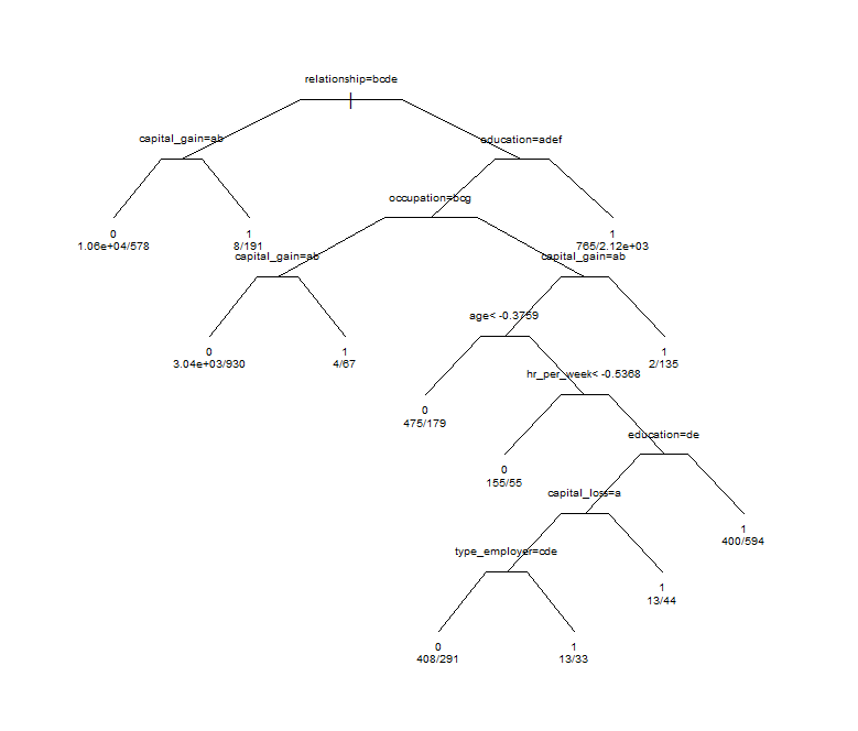We then prune with tree 8 as our target tree. To ensure we get tree 8, the CP value we give to the pruning algorithm is the geometric midpoint of CP values for tree 8 and tree 7.We can plot the tree in R using the plot command, but it’s a bit of work to get a good looking output.

par(mfrow = c(1, 1), mar = c(1, 1, 1, 1))
plot(prunedtree, uniform = T, compress = T, 
     margin = 0.1, branch = 0.3)
text(prunedtree, use.n = T, digits = 3, cex = 0.6)

We can now move to evaluating the fit. First we can generate the confusion matrix.

fit.preds = predict(prunedtree,newdata=data$val,type="class")
fit.table = table(data$val$income,fit.preds)
fit.table

Another way to check the output of the classifier is with a ROC (Receiver Operating Characteristics) Curve. This plots the true positive rate against the false positive rate, and gives us a visual feedback as to how well our model is performing. The package we will use for this is ROCR.

library(ROCR)
fit.pr = predict(prunedtree,newdata=data$val,type="prob")[,2]
fit.pred = prediction(fit.pr,data$val$income)
fit.perf = performance(fit.pred,"tpr","fpr")
plot(fit.perf,lwd=2,col="blue",
     main="ROC:  Classification Trees on Adult Dataset")
abline(a=0,b=1)

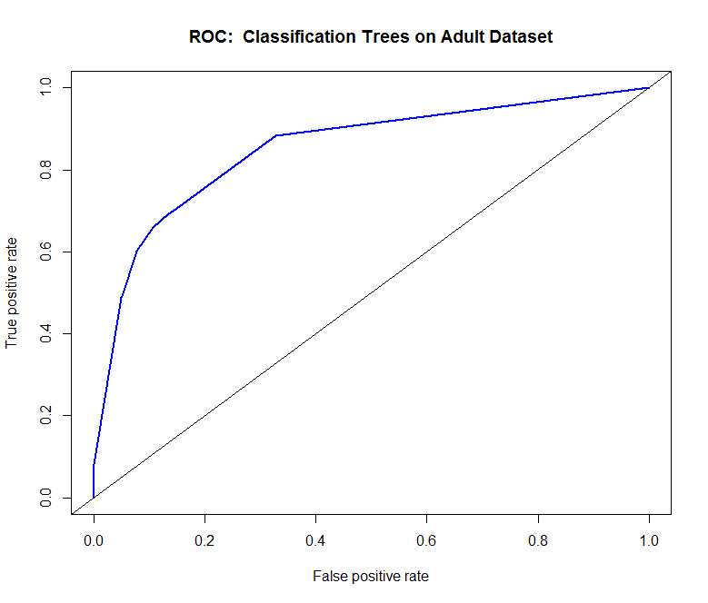Ordinarily, using the confusion matrix for creating the ROC curve would give us a single point (as it is based off True positive rate vs false positive rate). What we do here is ask the prediction algorithm to give class probabilities to each observation, and then we plot the performance of the prediction using class probability as a cutoff. This gives us the “smooth” ROC curve.

The full predict.rpart output from the model is a 2-column matrix containing class probabilities for both 0 (less than 50k) and 1 (greater than 50k) for each of the observations in the supplied dataset. Because the prediction() function expects simply the class probability of income being greater than 50k (IE, P(data$val$income == 1|model)), we need to supply only the second column.