Author Archives: Peter

Hypothesis Testing

Hypothesis testing allows us to evaluate a hypothesis, or compare two hypotheses. I include it here as part of the theoretical framework necessary for validation of the statistical models offered.

In hypothesis testing, there are two hypotheses.

$H_0$ is the null hypothesis. This is generally the hypothesis we are trying to disprove. We attempt to mount evidence against the null hypothesis.
$H_1$ is the alternative hypothesis. This is the hypothesis we are ready to accept if the null hypothesis is not rejected.

Types of Error – There are 2 types of error associated with hypothesis testing.

$\alpha$ is the probability of rejecting $H_0$ given $H_0$ is true.
is the probability of failing to reject given is false.
- Power of a test is given as $1-\beta$ . It is the probability of rejecting $H_0$ given $H_0$ is false.

A $p$ -value, associated with a test statistic, is the largest $\alpha$ -level at which we would still fail to reject the null hypothesis, given the data on hand. It is interpreted as the probability of seeing a sample (the data) as extreme or more extreme than what you saw, given $H_0$ (the null hypothesis) is true. We can NOT interpret the p-value as the likelihood that the null hypothesis is true. Data can not serve to prove the null hypothesis is true, data only offers evidence that it is untrue. We evaluate the strength of that evidence using the hypothesis test.

Example: Normal Hypothesis Testing, Known Variance, Unknown Mean
Let us assume that a sample of size $n$ is taken from a population with a known variance $\sigma^2$ , and unknown mean $\mu$ . We know this population to be normally distributed, so we can model the sample mean using a normal distribution without any further assumptions.

$\begin{align*} x_i : i = 1,\ldots,n &\sim N(\mu, \sigma^2)\\ \xbar = \frac{\sum_{i=1}^n x_i}{n} &\sim N(\mu,\frac{\sigma^2}{n})\\ \end{align*}$

Let’s say we have an initial guess as to the population mean, that we’re trying to disprove. We represent that with our null hypothesis. The alternative is given as the alternative hypothesis.

$H_0$ : $\mu = \mu_0$
$H_1$ : $\mu \neq \mu_0$

By nature of their definitions, we can’t calculate Power or $\beta$ levels without an actual value for $H_1$ , so I’m not going to here.

The test statistic for the normal distribution, $Z$ , is defined as $\frac{\xbar - \mu_0}{\sigma/\sqrt{n}}$ . $Z$ is normally distributed with mean 0 and variance 1. In this case, because we’re conducting a two-sided test, we calculate the rejection region of our test as being outside the range $(Z_{\frac{\alpha}{2}}, Z_{1-\frac{\alpha}{2}})$ . Depending on our intended level of significance, we go to the Z-table to get those values. If we use an $\alpha$ level of .05, then that range is approximately (-1.96, 1.96).

So if the $Z$ calculated from $Z=\frac{\xbar - \mu_0}{\sigma/\sqrt{n}}$ is greater than 1.96, or less than -1.96, then we reject the null hypothesis.

Example: Normal Hypothesis Testing, Unknown Variance
Let us assume we have a sample of size $n$ , taken from a population with an unknown variance $\sigma^2$ , and an unknown mean $\mu$ . We believe this population to be normally distributed, but since we don’t know the variance we can not use the normal model. Thus enters the Student’s T-test.

Because we don’t know the variance, we have to use an estimator of variance. The unbiased estimator of variance is $S^2 = \frac{\sum(x_i - \xbar)^2}{n-1}$ . We use $n-1$ degrees of freedom here because we subtract 1 for calculation of $\xbar$ .

Since we used an estimator of variance, we must use a different test statistic. Enter the $t$ statistic.

$\begin{equation*} T = \frac{\xbar - \mu_0}{S/\sqrt{n}} \sim t_{n-1} \end{equation*}$

The $T$ follows a student’s t distribution with $n-1$ degrees of freedom. The $t$ distribution itself asymptotically approaches the normal distribution as the degrees of freedom go up. In practice, it’s generally safe for sample sizes larger than 30 to simply use the normal distribution. However, because we’re performing calculations by computer, we can let the computer do the calculations and use the t distribution with however many degrees of freedom we have.

But anyways, we find the appropriate critical $t$ value for the given degrees of freedom, and $\alpha$ level. If $T$ as calculated by $T = \frac{\xbar - \mu_0}{S/\sqrt{n}}$ is less than $t_{\frac{\alpha}{2}, n-1}$ or greater than $t_{1-\frac{\alpha}{2},n-1}$ , then we reject the null hypothesis.

Classification Systems

Statistical classification involves the use of various methods and metrics to discriminate outcome variables into their correct groups using input variables. The algorithms used to do this are called classification systems, or classifiers. There are various metrics we use to gauge the performance of our classification systems. If we are referring exclusively to binary outputs, then we can use sensitivity, specificity, Positive and Negative Predictive Value, and correct classification percentage.

Accuracy is defined as the total number of correctly classified observations, divided by the total number of observations.

$\begin{equation*} \text{Accuracy} = \frac{\text{\# True Positives }+\text{ \# True Negatives}}{\text{Total \# of Observations}} \end{equation*}$

There exists some problems with this metric. If the condition we are trying to predict occurs at a rate nearing 1, then we can simply predict that all observations will be positive. This will give us a very strong accuracy, but obviously is not very good for prediction.

Positive Predictive Value is defined as the total number of correctly predicted positive outcomes from the test, divided by the total number of predicted positive outcomes (correctly predicted or not).

$\begin{equation*} PPV = \frac{\text{\# True Positives}}{\text{\# True Positives} + \text{\# False Positives}} \end{equation*}$

Negative Predictive Value is defined as the total number of correctly predicted negative outcomes, divided by the total number of predicted negative outcomes.

$\begin{equation*} NPV = \frac{\text{\# True Negatives}}{\text{\# True Negatives} + \text{\# False Negatives}} \end{equation*}$

Sensitivity, also called the True Positive Rate or Recall Rate, is defined as the total number of correctly predicted positive outcomes, divided by the total number of positive outcomes.

$\begin{equation*} \text{Sensitivity} = \frac{\text{\# True Positives}}{\text{\# True Positives} + \text{\# False Negatives}} \end{equation*}$

Specificity, also called the True Negative Rate, is defined as the total number of correctly predicted negative outcomes, divided by the total number of negative outcomes.

$\begin{equation*} \text{Specificity} = \frac{\text{\# True Negatives}}{\text{\# True Negatives} + \text{\# False Positives}} \end{equation*}$

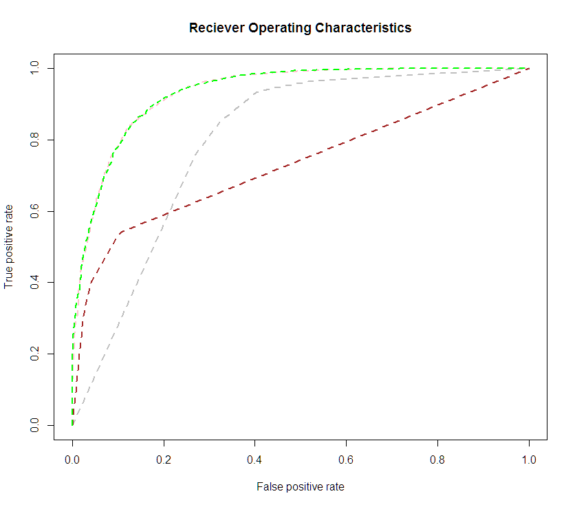
Reciever Operating Characteristics are a graphical representation of the performance of the classifier. The ROC curve is a two-dimensional plot with Sensitivity on the Y axis, $1 -$ Specificity on the X axis. The purpose is to observe how the sensitivity and specificity change as you vary the discrimination criteria. Most classification models will put out a value between 0 or 1 that represents the “odds” that that observation is a 1. the discrimination criteria is the cutoff point on that range (0,1) for which you declare that observation to be a 1. As you vary that cutoff point, you generate lines on the ROC curve. Then you pick the best cutoff point. In absence of other criteria for determining the best cutoff point, we will typically use the value that maximizes the lift, or distance between the observed sensitivity, specificity, and the diagonal line, where sensitivity is equal to specificity. This distance gives us a measure of how much better we’re doing than random guess.

The linked image is an example ROC curve from a paper where I was comparing classifier methods. Each color represents a method used. The closer the ROC curve gets to the upper left corner, the more powerful it is.

There is another metric associated with the ROC curve, called the area under the curve. If we calculate the Area under the curve, or AUC, we get a number somewhere between 0 and 1. At first glance, this might seem a useful method of comparing two classifier methods, since holding the shape of the curves constant, a higher AUC indicates a more powerful classifier. However, the AUC ignores where along the ROC curve we might want that power. If we can tolerate a false positive rate of only so high, then we have to make comparisons in lift at those thresholds, rather than calculating a single metric like AUC.

Additional Resources:
Wikipedia – Confusion Matrix – Worked Example
SaedSayed – Model Evaluation

Rstudio, Sweave, and LaTeX

$\text{\LaTeX}$ (pronounced Lay-tech, the X is supposed to be a capital $\chi$ ) is a typesetting environment used to generate a professional looking output, and automate some of the more tedious tasks of writing a paper. It is the de-facto standard for writing scientific papers, and it is a good idea to learn it if you intend to release academically. Also, if you’ve been frustrated fiddling with Microsoft’s Equation Editor for writing your papers, LaTeX will alleviate your pain.

Rstudio is an integrated development environment for the R statistical programming language. It makes most programming tasks with R much easier and more productive. Packaged in Rstudio are plugins that allow for the merging of R output (code, data, graphs) and the typesetting abilities of $\text{\LaTeX}$ . To take advantage of this, you will additionally need a $\text{\LaTeX}$ Installation. The one I will recommend here is MiKTeX.

R: http://cran.stat.ucla.edu/
Rstudio: http://www.rstudio.com/ide/download/
MiKTeX: http://miktex.org/download

These recommendations are of course based on the user using Microsoft Windows. If that is not the case, then for using Linux the recommendation changes to TeXLive or teTeX. The Mac recommendation is MacTeX. There are some differences between the distributions in what they will support. A document that compiles without issue on one may not compile on another.

Sweave
Sweave is the transition piece between R and LaTeX. Named for S-Weave (S being the closed-source statistical language R is emulating), Sweave “weaves” R code and output into LaTeX documents. Within Rstudio, you create a Sweave document (with the .Rnw extension) and encapsulate R code into “chunks”. Within those chunks, any R code can be run, and output presented as R natively would. Below is a sample .Rnw file to demonstrate this.

\documentclass{article}
# options for the document go here.
# load LateX packages, declare new macros
\begin{document}

<<>>=
# this is an R code chunk.  R code goes in here, 
# between the angle brackets and the at symbol.
a = 123456
print(a)
@
This will declare the variable a and print it as R would, 
within the R chunk.  If we want to output the results of R 
inline into document text, then we can do so with Sexpr.  
The content of the variable a is \Sexpr{a}.
\end{document}

Within the code chunk declaration, we can set various options for the chunk. If we intend to have the chunk make a plot, we would need to declare fig=TRUE within the chunk declaration. If we intend to hide the code used, but still let it run, then we set echo=FALSE. If we don’t intend the code to run, merely display it, then we would use eval=FALSE. There are many other options available for our use.

Additional Links

A Sweave Demo – Charles Geyer, UMN. An excellent demonstration on the document preparation abilities of Sweave, and incorporating R output with a LateX document
LaTeX User Guide – An unofficial user guide for how to $\text{\LaTeX}$
LaTeX Math Symbols – A list of common (and not so common) mathematical symbols in LaTeX

R Environment

R is one of the more commonly used statistical analysis software. The ease with which methods can be prototyped and brought to production makes it very popular for research. The fact that it is open source, and free to use also contributes to its appeal.

The official manual for R is available here. I recommend reading at least some of it to get used to the language. If this is your first programming language, a small foray into python using google’s online python class might also do some good.

There are IDE’s (Integrated Development Environments) to use with R to make your life easier. Of these, the one I recommend is Rstudio. The use of an IDE is optional, but if you do a lot of coding it will make your life easier.

The official websites are as follows:

R – http://www.r-project.org/

Rstudio – http://www.rstudio.com/

Using Rstudio also gives you easy access to the document publishing abilities of $\text{\LaTeX}$ . Within Rstudio, you can encapsulate R code into “chunks”, which will generate results and be placed into the typeset paper. This is made possible with plugins in Rstudio called Sweave or knitr. See more on the appropriate tutorial page.

Multiple Linear Regression

Multiple Linear Regression (MLR) allows us to find a linear relationship between multiple input variables and a single dependent output variable. This tutorial is going to be given in matrix notation. For more on matrix notation, including the rules of matrix multiplication, I suggest visiting the wikipedia page on the subject here. We are again going to have to define some additional notation.

$n$ is the number of observations in the data set.
$p$ is the number of predictor variables used in the regression.
$Y_{n\times 1}$ is the vector of dependent variable observations. It is $n$ observations long, 1 variable wide.
$X_{n\times p'}$ is the matrix of dependent variables. It includes a vector of 1’s as the first column to represent the intercept. Its dimensions are $n$ observations long, and $p' = p+1$ observations wide. (Note: If we are purposely not including the intercept in the model, then we omit the leading vector of 1’s, and the dimensions of $X$ are $n \times p$ .)
$\beta_{p'\times 1}$ is the vector of coefficients. Its dimensions are $p'=p+1$ long, 1 wide. (Also note: If not including the intercept, $\beta_0$ is dropped, and the dimensions of $\beta$ are $p\times 1$ .)
$\err_{n\times 1}$ is the vector of errors.

I will not be keeping up the subscript notation all the way through this tutorial. Just remember that it is there. The model in multiple linear regression in matrix form is as follows:

$\begin{equation*} Y = X\beta + \err \end{equation*}$

Expanded, it appears as

$\begin{equation*} \begin{bmatrix} y_{1} \\ y_2\\ \vdots \\ \y_n\\ \end{bmatrix} = \begin{bmatrix} 1 & x_{1,1} & \cdots & x_{1,p} \\ 1 & x_{2,1} & \cdots & x_{2,p} \\ \vdots & \vdots & \ddots &\vdots \\ 1 & x_{n,1} & \cdots & x_{n,p} \\ \end{bmatrix} \begin{bmatrix} \beta_0 \\ \beta_1 \\ \vdots \\ \beta_p \\ \end{bmatrix} + \begin{bmatrix} \err_{1}\\ \err_{2}\\ \vdots\\ \err_{n}\\ \end{bmatrix} \end{equation*}$

Deriving The $\beta$ Vector

We are still using Ordinary Least Squares (OLS) regression, so we will use the assumptions of that to generate the estimates of the coefficients. Because we don’t know what the actual errors are, the observed errors will be denoted by an $e$ . So we want to minimize $\sum(e^2) = e'e$ .

$\begin{align*} e'e &= (Y-X\bhat)'(Y-X\bhat)\\ &= Y'Y - \bhat'X'Y - Y'X\bhat + \bhat'X'X\bhat\\ &= Y'Y - 2\bhat'X'Y + \bhat'X'X\bhat \end{align*}$

Take the derivative with respect to $\bhat$ to yield

$\begin{equation*} \frac{\partial e'e}{\partial \bhat} = -2X'Y + 2X'X\bhat = 0 \end{equation*}$

This gives us the ‘Normal Equations’.

$\begin{equation*} X'X\bhat = X'Y \end{equation*}$

If the inverse of $X'X$ exists, then we can solve the normal equations, yielding our estimator for $\beta$ , $\bhat$ .

$\begin{align*} (X'X)^{-1}(X'X)\bhat &= (X'X)^{-1}X'Y\\ \bhat &= (X'X)^{-1}X'Y \end{align*}$

Now, This gives us the estimator for $\beta$ . We need to verify that it is unbiased, and develop the variance of this estimator.

$\begin{align*} \bhat &= [(X'X)^{-1}X']Y\\ E(\bhat) &= [(X'X)^{-1}X']E(Y)\\ &=(X'X)^{-1}(X'X)\beta\\ &=\beta \end{align*}$

So the estimator is unbaised. The Variance can be calculated as follows.

$\begin{align*} Var(\bhat) &= [(X'X)^{-1}X']Var(Y)[(X'X)^{-1}X']'\\ &= [(X'X)^{-1}X']I\sigma^2[(X'X)^{-1}X']'\\ &= (X'X)^{-1}\sigma^2 \end{align*}$

So, $\bhat \sim N(\beta,(X'X)^{-1}\sigma^2)$ . This will be necessary for estimating the Confidence Interval

Confidence Interval for $\bhat$
The Confidence Interval for $\bhat$ is derived from the relationship between the normal distribution an the Student’s T distribution. The Confidence Interval for any element of the $\bhat$ vector, $\bhat_j$ can be defined as

$\begin{equation*} 100(1-\alpha)\%\text{ CI }\bhat_j = \bhat_j \pm t_{\frac{\alpha}{2},n-p'}SC_{jj} \end{equation*}$

Where $S$ is the sample standard deviation of the residuals, and $C_{jj}$ is the jj’th element of $(X'X)^{-1}$

The Hat (or Projection) Matrix
The projection matrix will be important later on. For now, let us derive it.

$\begin{align*} \yhat &= X\bhat\\ &= X[(X'X)^{-1}X'Y]\\ &= [X(X'X)^{-1}X']Y\\ &= PY\\ P &= [X(X'X)^{-1}X'] \end{align*}$

Simple Linear Regression

Simple linear regression seeks to find a linear relationship between two variables; the independent ‘predictor’ variable, and the dependent ‘outcome’ variable. We represent this linear relationship with a line, the slope of which allows us to make inferences as to the nature of the relationship. I.e., for every unit change in the predictor variable, the outcome variable changes by this amount.

The most commonly used method of creating that line is called “Ordinary Least Squares” (OLS). It is called this, because we try to minimize the sum of the squared residuals. Before this gets too in depth, we should define some terms.

The mean of a variable is the sum of all observations of that variable, divided by the number of observations.
$x_i$ is the $i$ th observation of the variable $x$ .
$y_i$ is the $i$ th observation of variable $y$ .
${\bar x}$ is the mean of the predictor variable $x$ .
${\bar y}$ is the mean of the outcome variable $y$ .
${\hat y}_i$ is the predicted value for variable $y$ at observation $i$ .
$\varepsilon_i$ is the residual, or distance from the fitted value ${\hat y}$ and the actual value $y$ at observation $i$ .

In order to use OLS, we must make a few assumptions as to the nature of the residuals. We must assume that the residuals are normally distributed (follow the normal or Gaussian distribution) with a mean of 0, and a constant variance (homoscedastiscity). There are more complex regression techniques that relax these assumptions that we will not be delving into here.

A number that scales a variable is called a ‘coefficient’. A number that stands alone is called a constant.

$\beta_0$ is a constant, and represents the y-intercept of the line. $\beta_1$ is a coefficient, and expresses the linear relationship between $y$ and $x$ . We represent the line we intend to draw with the equation:

$\begin{equation*} y_i = \beta_0 + \beta_1 x_i + \err_i \end{equation*}$

Calculating the Coefficients

By using the ordinary least squares approach, we choose to minimize the sum of squared residuals.

$\begin{equation*} \min(Q_{(\beta_0,\beta_1)}) \text{ where }Q_{(\beta_0,\beta_1)} = \sum_{i=1}^{n}\varepsilon_i^2 = \sum_{i=1}^n(y_i - \beta_0 - \beta_1x_i)^2 \end{equation*}$

Using Calculus, we can differentiate $Q_{(\beta_0,\beta_1)}$ on $\beta_0$ and $\beta_1$ , set the results equal to 0 and solve for $\beta_0$ and $\beta_1$ . This yields our resulting estimators.

$\begin{equation*} {\hat \beta}_0 = {\bar y} - {\hat \beta}_1 {\bar x} \hspace{1cm}{\hat \beta}_1 = \frac{\sum_{i=1}^n(y_i - {\bar y})(x_i - {\bar x})}{\sum_{i=1}^n(x_i - {\bar x})^2} \end{equation*}$

Up till now, none of this has required any assumptions as to the nature of the errors. Continuing on, we intend to make inferences and declare validity of the model, and for that we will need the assumption of normality of residuals.

Significance of the Regression

After generating a model, we test whether that model is significant.

$\begin{align*} &H_0\text{: }\beta_1 = 0\text{ - The regression is not significant}\\ &H_1\text{: }\beta_1 \neq 0 \text{ - The regression is significant}\\ \end{align*}$

The statistic for this test follows the student’s t-test with degrees of freedom $n-2$ .

$\begin{equation*} T = \frac{\bhat_1 - 0}{SE(\bhat_1)} \hspace{2cm}SE(\beta_1)\sim t_{n-2} = \sqrt{\frac{\frac{1}{n-2}\sum_{i=1}^n\err_i^2}{\sum_{i=1}^n(x_i-\xbar)^2}} \end{equation*}$

Assuming the errors are normally distributed, this allows us to make several inferences. First, we can check whether the regression model is valid. To do that, we have to use the standard 2-sided hypothesis testing detailed in the hypothesis testing section. We’re using a t-distribution with $n-2$ degrees of freedom.

$\begin{align*} H_0\text{: }\beta_1 = 0\\ H_1\text{: }\beta_1 \neq 0\\ \end{align*}$

So we calculate the $t$ statistic for $\bhat_1$ , and find the associated $p$ value to that statistic. If the $p$ value is less than $\alpha$ , then we reject the null hypothesis and declare the regression model valid. For completeness sake, the standard Error of $\bhat_0$ can be calculated as:

$\begin{equation*} SE(\bhat_0) = \sqrt{\sigma^2(\frac{1}{n} + \frac{\xbar^2}{\sum_{i=1}^n(x_i - \xbar)^2})} \end{equation*}$

Confidence Intervals

Using the derivations of the standard errors of the coefficients, and using the t-distribution nature of them, we can generate confidence interval around $\beta_0$ and $\beta_1$ such that we are $100(1-\alpha)\%$ sure the true regression coefficients lie within those bounds.

$\begin{align*} 100(1-\alpha)\%\text{ CI }\beta_1 &= \bhat_1 \pm t_{\frac{\alpha}{2}}*SE(\bhat_1)\\ 100(1-\alpha)\%\text{ CI }\beta_0 &= \bhat_0 \pm t_{\frac{\alpha}{2}}*SE(\bhat_0)\\ \end{align*}$

Similarly, given the values, variances and covariances for the beta coefficients, we can generate confidence intervals for the predicted values (or means) of new $y$ values for a given $x_{new}$ .

$\begin{align*} 100(1-\alpha)\%\text{ CI }\yhat_{new} &= \bhat_0 + x_{\new}\bhat_1 \pm t_{\frac{\alpha}{2}}*SE(\yhat_{new})\\ SE(\yhat_{new}) &= \sqrt{\frac{1}{n} + \frac{(x_{new}-\xbar)^2}{\sum_{i=1}^{n}(x_i - \xbar)^2}} \end{align*}$

Prediction Intervals
While confidence intervals give boundaries for the parameters of the regression line, prediction intervals operate slightly differently. With prediction intervals, we are $100(1-\alpha)\%$ sure that new observations will fall within the prediction lines. In other words, we’re not just accounting for the variance of the estimated parameters, but also for the variance of the observation itself. This has a quick and rather handy interpretation of simply adding the variances of the confidence interval and the error of the observation itself to form a new variance term.

$\begin{align*} 100(1-\alpha)\%\text{ PI } y_{new} &= \bhat_0 + x_{new}\bhat_1 \pm t_{\frac{\alpha}{2},n-2}SE(y_{new})\\ SE(y_{new}) &= \sqrt{1 + \frac{1}{n} + \frac{(x_{new} - \xbar)^2}{\sum_{i=1}^n(x_i-\xbar)^2}} \end{align*}$

Statistical Consulting Group

San Diego State University