Logistic Regression is a type of classification model. In classification models, we attempt to predict the outcome of categorical dependent variables, using one or more independent variables. The independent variables can be either categorical or numerical.
Logistic regression is based on the logistic function, which always takes values between 0 and 1. Replacing the dependent variable of the logistic function with a linear combination of dependent variables we intend to use for regression, we arrive at the formula for logistic regression.

We can interpret  as the probability
  . I.e., the probability that the dependent variable is of class 1, given the independent variables.
For this tutorial, we will be performing logistic regression on the “Adult” dataset. I have previously explained the data preparation and transformations that I use for this dataset in this tutorial. We can import the dataset and repeat the transformations using the provided source file.
source("https://scg.sdsu.edu/wp-content/uploads/2013/09/dataprep.r")
To fit the logistic regression model, we will use the glm method. This is available in vanilla R without any other packages necessary. However, some packages provide more options for model fitting and model diagnostics than is available here. I also recommend the rms package, as it contains natively many different diagnostic tests for all sorts of regression.
fit1 = glm(income ~ ., family = binomial(logit), data = data$train)
Here for the formula, I am fitting income versus all other variables in the data frame. glm expects a family, which asks for the family of the error function, and the type of link function. Here I’m using Binomial errors, and the link function is logit, for logistic regression.
fit1sw = step(fit1) # Keeps all variables
the step() function iteratively tries to remove predictor variables from the model in an attempt to delete variables that do not significantly add to the fit. The stepwise model selection schema was covered in the regression schema tutorial. It is unchanged in this application.
It is interesting to note here that by AIC, the stepwise model selection schema kept all variables in the model. We will want to choose another criteria to check the variables included. A good choice is the variable inflation factor.
The variable inflation factor in the car package provides a useful means of checking multicollinearity. Multicollinearity is what happens when a given predictor in the model can be approximated by a linear combination of the other predictors in the model. This means that your inputs to the model are not independent of each other. This has the effect of increasing the variance of model coefficients. We want to decrease the variance to make our models more significant, more robust. That’s why it’s a good idea to omit variables from the model which exhibit a high degree of multicollinearity.
The VIF for a given predictor variable can be calculated by taking a linear regression of that predictor variable on all other predictor variables in the model. From that fit, we can pull an  value. The VIF is then calculated as

where VIF is the variable inflation factor for variable  ,
,  is the Coefficient of Determination for a model where the th variable is fit against all other predictor variables in the model. In this case, because we’re using logistic regression, the car package implements a slightly different VIF calculation called GVIF, or generalized VIF. The interpretation is similar. On normal VIF in multiple regression, we attempt to eliminate variables with a VIF higher than 5.
library(car)
vif(fit1)
We see from the output of the VIF function, that the variables marital, and relationship are heavily collinear. We will eliminate one of them from the model. I will choose relationship, as its meaning is somewhat difficult to understand, and thus limits our ability to interpret the model. We will now fit the new model using the glm() function.
fit2 = glm(income ~.-relationship, family = binomial(logit),
       data = data$train)
vif(fit2)
VIF for fit2 finds no variables with a high VIF. Therefore the model passes the multicollinearity test. There are a few other tests we can give the model before declaring it valid. The first is the Durbin Watson test, which tests for correlated residuals (An assumption we make is for non-correllated residuals). We can also try the crPlots() function. It plots the residuals against the predictors, allowing us to see which categorical variables contributed the most to variance, or allowing us to spot possible patterns in the residuals on numerical variables.
durbinWatsonTest(fit2)
crPlots(fit2)
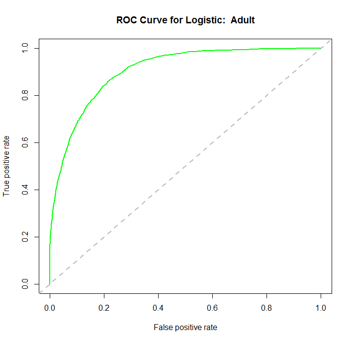
With a Durbin Watson statistic of 1.975, an associated p-value of .096, we fail to reject the null hypothesis, that the errors are correllated. We can call the model valid. But we do have one more means of testing the overall fit of the model, and that is empirical justification. We will see how well the model predicts on new data. In the dataprep() function called in the source(…) line, we split the complete dataset into 2 parts: the training dataset, and the validation dataset. We will now predict based on the validation dataset, and use those predictions to build a ROC curve to assess the performance of our model.
library(ROCR)
fitpreds = predict(fit2,newdata=data$val,type="response")
fitpred = prediction(fitpreds,data$val$income)
fitperf = performance(fitpred,"tpr","fpr")
plot(fitperf,col="green",lwd=2,main="ROC Curve for Logistic:  Adult")
abline(a=0,b=1,lwd=2,lty=2,col="gray")
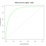 We can see that the performance of the model rises well above the diagonal line, indicating we are doing much better than random guess. As to how well this particular model fares against other models, we would need to compare their ROC curves using the same datasets for training and validation.

 statistics test significance of point estimates for slope and intercept, while the
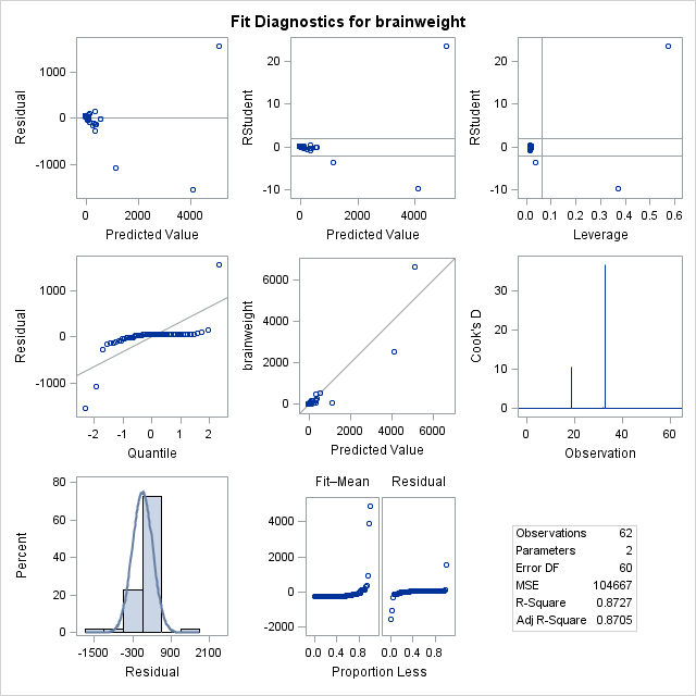
  statistic is the overall significance of the regression. They say that the regression is significant, so that there is a linear effect. However, none of these statistics accurately capture what is wrong with this fit. Look at the diagnostic plots, the fitted vs residual plots, and the QQ plot. They warn of something very wrong here. In the “Quantile to Quantile” (or QQ) plot, we see how closesly the residuals from the fit match a normal distribution. They don’t. Given that one of the assumptions of least squares linear regression is that the residuals follow a normal distribution, we can see we have a problem here. We can also see this by the histogram of residuals on the bottom, with a superimposed normal curve. It is clear to see that the residuals do not follow a normal distribution. To fix this, one thing we can do to make a valid model is to attempt transformations of the variables. A reasonable choice might be a log transform of the independent variable.
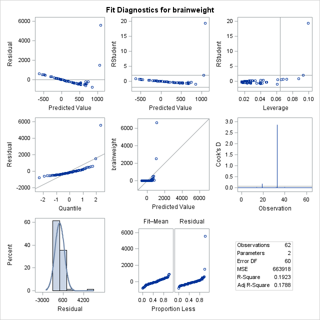
 ‘s, we can see that the regression is still significant. However, the transformation actually makes the fit significantly worse. We see a clear pattern in the residuals, and a QQ plot that appears almost flat where it should be diagonal. Considering that log transforming the dependent variable without transforming the independent variable would just skew the data the other way, another choice we have would be to log transform both independent and dependent variables.
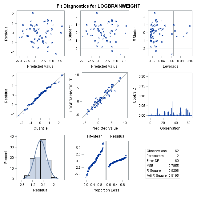
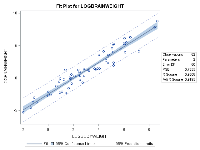
 , we get this.
 is a binary variable, taking values of either
  . The predictor (or input, or independent) variables
  are not limited in this way, and can take any value.
 is the vector of independent variable observations for subject
  .
.  . I.e., the probability that the dependent variable is of class 1, given the independent variables.
 is the probability of an event occuring.
  is the probability of that event not occuring. Odds is defined as
  . IE, the ratio of probabilities of that event occuring over that event not occuring.
 . So now, we declare the logit equal to the linear combination of covariates.
 . We can solve this using the least squared error solution from linear regression.
 with replacement from the original dataset. The goal is that iteratively drawing from the existing sample, we can simulate new draws from the population. Aggregation refers to aggregating the class votes from the models trained on each of the bootstrap samples.
 (the number of bootstrap samples)
 :
: 

 concept. At each split, rather than trying every possible split on every variable, we randomly select