Multiple Linear Regression (R) | Statistical Consulting Group

In this tutorial, we are going to be walking through multiple linear regression, and we are going to recognize that it’s not a lot different than simple linear regression.

The model in multiple linear regression looks similar to that in simple regression. We’re adding more coefficients to modify the additional independent variables.

$\begin{equation*} Y_{i} = \beta_0 + \beta_1X_{i,1} + \beta_2X_{i,2} + \ldots + \beta_pX_{i,p} + \err_i \hspace{1cm} \err_i \sim N(0,\sigma^2) \end{equation*}$

url="https://scg.sdsu.edu/wp-content/uploads/2013/09/drinking.txt"
data = read.table(url,skip=41,header=F)
names(data) = c("Index","One","pop","lb","wine","liquor","cirrhosis")

We skip the first 41 rows of the file due to it being descriptions of the data and not the data itself. Because variable names aren’t conveneniently placed on a single line, we name the columns by hand with the name() function.

We set up an ititial fit.

fit1 = lm(cirrhosis~pop+lb+wine+liquor,data=data)

To see an initial reduced model, we can use stepwise model selection to pare down the non-significant predictors. There are various criteria to determine which model we use is the “best”, but one of the more commonly used ones is Akaike’s Information Criterion, or AIC.

$\begin{equation*} \text{AIC} = 2p - 2\ln(L) \end{equation*}$

Where $p$ is the number of coefficients being calculated, and $L$ is the maximized value of the likelihood function for the model. AIC effectively penalizes a model for using too many predictor variables, so we only include more predictor variables if they significantly increase the model’s likelihood function. That is, only if they lend sufficient additional information to the model to justify their inclusion.

library(MASS)
fit1sw = stepAIC(fit1)
summary(fit1sw)

We probably should have checked this prior to now, but it’s a good idea to check the pairwise plots of the independent versus dependent variables at some point to look for any obvious transformations we could make.

par(mfrow=c(2,2))
plot(x=data$pop,y=data$cirrhosis,xlab="population",ylab="cirrhosis")
plot(x=data$lb,y=data$cirrhosis,xlab="lower births",ylab="cirrhosis")
plot(x=data$wine,y=data$cirrhosis,xlab="wine",ylab="cirrhosis")
plot(x=data$liquor,y=data$cirrhosis,xlab="liquor",ylab="cirrhosis")

We don’t really see any obvious transformations we could make that would increase the linearity of the regressors. In like manner, there’s no obvious transformations we can make to the dependent variable to form a better regression.
As such, we have the option to stop here and take a look at the diagnostic plots of the reduced model.

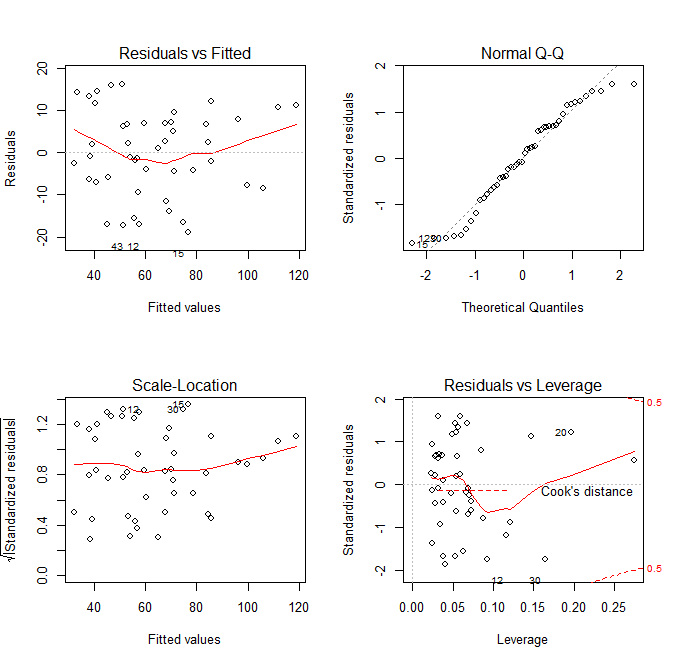
Here we see the diagnostic plots of the reduced model. We don’t see any obvious pattern to the residuals, but there is some worrying deviation from the diagonal line on the QQ plot. In the Cook’s Distance plot, we’re ideally hoping that no observations have a Cooke’s Distance greater than .10. Clearly that’s not the case.

In looking at the summary of the fitted model, we can see that the final relationship given comes out to being:

$\begin{equation*} y_i = -16.0008 + 1.3656*\text{lb}_i + 1.9723*\text{wine}_i + \err_i \hspace{.5cm} \err_i \sim N(0,10.38^2) \end{equation*}$

The Coefficient of Determination gives the percentage change in the dependent variable $y$ caused by change in the independent variables lb and wine. In the summary, we see it as .8128, meaning 81% of the change in the cirrhosis variable can be “explained by” changes in the independent variables in the fit.

The F statistic is given for an overall hypothesis test,

H $_0$ : $\beta_i = 0$ for all $i$ . In this case, $\beta_1,\beta_2 = 0$ , meaning that neither wine nor lb have a linear effect on cirrhosis.
H $_1$ : $\beta_i \neq 0$ for some $i$ . In this case, at least one of $\beta_1,\beta_2$ does not equal 0, meaning that there is a linear effect on cirrhosis for at least one of the predictors.

The F statistic given in the summary is 93.34, on 2 and 43 degrees of freedom. That gives a P-value very close to 0, meaning we would reject the null hypothesis. The regression is significant.

shapiro.test(fitsw$resid)

The final test for the fitted model is a test of normality of errors. The Shapiro-Wilk Normality Test will test whether the residuals of the fitted model follow a normal distribution. The hypotheses for this test are given as follows:

H $_0$ : $\err_i \sim N(0,\sigma^2)$ – The errors follow a normal distribution
H $_1$ : $\err_i \not\sim N(0,\sigma^2)$ – The errors do not follow a normal distribution

If we reject the null hypothesis, then we have disproved one of the base assumptions we make for linear regression. Therefore, we are hoping to not reject the null hypothesis. The output statistic from the Shapiro-Wilk test is $w=.9579$ , with an associated p-value of $.0953$ . Being that $.0953 > .05$ , the $\alpha$ level we typically use for these tests, we fail to reject the null hypothesis. We can regard the errors as normal, satisfying the assumption of the regression. We can call the fit valid.